7 Scenario VI: binomial distribution

7.1 Details

In this scenario, the implemented normal approximation of the binomial distribution is evaluated. There are two treatment groups \(E\) (experimental) and \(C\) (control) and the outcome of interest is the event rate in both groups. The event rate in the control group is assumed to equal \(p_C = 0.3\). Under the null hypothesis, the rate difference \(p_E - p_C = 0\) is assumed. Under the alternative, the rate difference is assumed to equal \(p_E - p_C = 0.2\). Type one error rate should be protected at 2.5% and the design’s power should be at least 90%.

# data distribution and hypotheses
datadist   <- Binomial(rate_control = 0.3, two_armed = TRUE)
H_0        <- PointMassPrior(.0, 1)
prior      <- PointMassPrior(.2, 1)

# define constraints
alpha      <- 0.025
min_power  <- 0.9
toer_cnstr <- Power(datadist, H_0)   <= alpha
pow_cnstr  <- Power(datadist, prior) >= min_power

7.2 Variant VI-1, efficiency of optimal designs for binomial distribution

In this variant, it is evaluated whether the optimization leads to more efficient designs and is plausible with published results.

7.2.1 Objective

Expected sample size under the alternative point mass prior \(\delta = 0.2\) is minimized.

ess <- ExpectedSampleSize(datadist, prior)

7.2.2 Constraints

No additional constraints are considered.

7.2.3 Initial Designs

For this example, the optimal one-stage, group-sequential, and generic two-stage designs are computed. The initial design for the one-stage case is determined heuristically and both the group sequential and the generic two-stage designs are optimized starting from the corresponding group-sequential design as computed by the rpact package.

order <- 7L
# data frame of initial designs 
tbl_designs <- tibble(
    type    = c("one-stage", "group-sequential", "two-stage"),
    initial = list(
        OneStageDesign(200, 2.0),
        rpact_design(datadist, 0.2, 0.025, 0.9, TRUE, order),
        TwoStageDesign(rpact_design(datadist, 0.2, 0.025, 0.9, TRUE, order))) )

The order of integration is set to 7.

7.2.4 Optimization

tbl_designs <- tbl_designs %>% 
    mutate(
       optimal = purrr::map(initial, ~minimize(
         
          ess,
          subject_to(
              toer_cnstr,
              pow_cnstr
          ),
          
          initial_design = ., 
          opts           = opts)) )

7.2.5 Test Cases

To avoid improper solutions, it is first verified that the maximum number of iterations was not exceeded in any of the three cases.

tbl_designs %>% 
  transmute(
      type, 
      iterations = purrr::map_int(tbl_designs$optimal, 
                                  ~.$nloptr_return$iterations) ) %>%
  {print(.); .} %>% 
  {testthat::expect_true(all(.$iterations < opts$maxeval))}

## # A tibble: 3 × 2
##   type             iterations
##   <chr>                 <int>
## 1 one-stage                28
## 2 group-sequential       1774
## 3 two-stage              4736

Next, the type one error rate and power constraints are verified for all three designs by simulation:

tbl_designs %>% 
  transmute(
      type, 
      toer  = purrr::map(tbl_designs$optimal, 
                         ~sim_pr_reject(.[[1]], .0, datadist)$prob), 
      power = purrr::map(tbl_designs$optimal, 
                         ~sim_pr_reject(.[[1]], .2, datadist)$prob) ) %>% 
  unnest(., cols = c(toer, power)) %>% 
  {print(.); .} %>% {
  testthat::expect_true(all(.$toer  <= alpha * (1 + tol)))
  testthat::expect_true(all(.$power >= min_power * (1 - tol))) }

## # A tibble: 3 × 3
##   type               toer power
##   <chr>             <dbl> <dbl>
## 1 one-stage        0.0251 0.900
## 2 group-sequential 0.0249 0.900
## 3 two-stage        0.0249 0.901

Since the degrees of freedom of the three design classes are ordered as ‘two-stage’ > ‘group-sequential’ > ‘one-stage’, the expected sample sizes (under the alternative) should be ordered in reverse (‘two-stage’ smallest). Additionally, expected sample sizes under both null and alternative are computed both via evaluate() and simulation-based.

ess0 <- ExpectedSampleSize(datadist, H_0)
tbl_designs %>% 
    mutate(
        ess      = map_dbl(optimal,
                           ~evaluate(ess, .$design) ),
        ess_sim  = map_dbl(optimal,
                           ~sim_n(.$design, .2, datadist)$n ),
        ess0     = map_dbl(optimal,
                           ~evaluate(ess0, .$design) ),
        ess0_sim = map_dbl(optimal,
                           ~sim_n(.$design, .0, datadist)$n ) ) %>% 
    {print(.); .} %>% {
    # sim/evaluate same under alternative?
    testthat::expect_equal(.$ess, .$ess_sim, 
                           tolerance = tol_n,
                           scale = 1)
    # sim/evaluate same under null?
    testthat::expect_equal(.$ess0, .$ess0_sim, 
                           tolerance = tol_n,
                           scale = 1)
    # monotonicity with respect to degrees of freedom
    testthat::expect_true(all(diff(.$ess) < 0)) }

## # A tibble: 3 × 7
##   type             initial    optimal          ess ess_sim  ess0 ess0_sim
##   <chr>            <list>     <list>         <dbl>   <dbl> <dbl>    <dbl>
## 1 one-stage        <OnStgDsg> <adptrOpR [3]> 124     124   124      124  
## 2 group-sequential <GrpSqntD> <adptrOpR [3]>  96.2    96.2  89.7     89.8
## 3 two-stage        <TwStgDsg> <adptrOpR [3]>  94.3    94.2  98.5     98.6

The expected sample size under the alternative must be lower or equal than the expected sample size of the initial rpact group-sequential design that is based on the inverse normal combination test.

testthat::expect_lte(
  evaluate(ess, 
             tbl_designs %>% 
                filter(type == "group-sequential") %>% 
                pull(optimal) %>% 
                .[[1]]  %>%
                .$design ),
    evaluate(ess, 
             tbl_designs %>% 
                filter(type == "group-sequential") %>% 
                pull(initial) %>% 
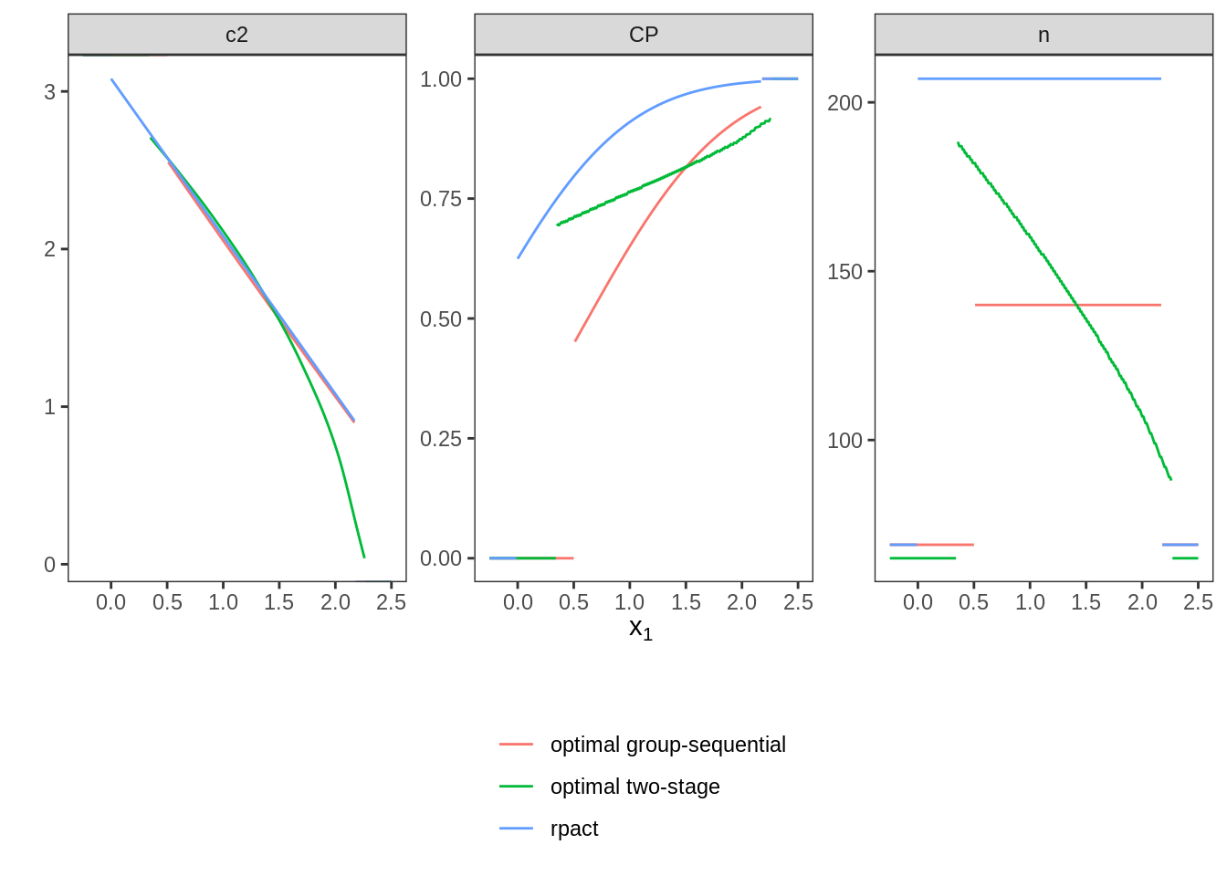
                .[[1]] ) )

Finally, the rpact group-sequential design, the optimal group-sequential design, and the optimal generic two-stage design are plotted to allow visual inspection.