2 Scenario I: large effect, point prior

2.1 Details

In this scenario, a classical two-arm trial with normal test statistic and known variance (w.l.o.g. variance of the test statistic is 1). This situation corresponds to a classical \(z\)-test for a difference in population means. The null hypothesis is no population mean difference, i.e. \(\mathcal{H}_0:\delta \leq 0\). An alternative effect size of \(\delta = 0.4\) with point prior distribution is assumed. Across all variants in this scenario, the one-sided maximal type one error rate is restricted to \(\alpha=0.025\) and the power at the point alternative of \(\delta=0.4\) must be at least \(0.8\).

# data distribution and hypotheses
datadist   <- Normal(two_armed = TRUE)
H_0        <- PointMassPrior(.0, 1)
prior      <- PointMassPrior(.4, 1)

# define constraints
alpha      <- 0.025
min_power  <- 0.8
toer_cnstr <- Power(datadist, H_0)   <= alpha
pow_cnstr  <- Power(datadist, prior) >= min_power

2.2 Variant I-1: Minimizing Expected Sample Size under Point Prior

2.2.1 Objective

Firstly, expected sample size under the alternative (point prior) is minimized, i.e., \(\boldsymbol{E}\big[n(\mathcal{D})\big]\).

ess <- ExpectedSampleSize(datadist, prior)

2.2.2 Constraints

No additional constraints besides type one error rate and power are considered in this variant.

2.2.3 Initial Designs

For this example, the optimal one-stage, group-sequential, and generic two-stage designs are computed. The initial design for the one-stage case is determined heuristically (cf. Scenario III where another initial design is applied on the same situation for stability of initial values). Both the group sequential and the generic two-stage designs are optimized starting from the corresponding group-sequential design as computed by the rpact package.

order <- 7L
# data frame of initial designs 
tbl_designs <- tibble(
    type    = c("one-stage", "group-sequential", "two-stage"),
    initial = list(
        OneStageDesign(200, 2.0),
        rpact_design(datadist, 0.4, 0.025, 0.8, TRUE, order),
        TwoStageDesign(rpact_design(datadist, 0.4, 0.025, 0.8, TRUE, order))) )

The order of integration is set to 7.

2.2.4 Optimization

tbl_designs <- tbl_designs %>% 
    mutate(
       optimal = purrr::map(initial, ~minimize(
         
          ess,
          subject_to(
              toer_cnstr,
              pow_cnstr
          ),
          
          initial_design = ., 
          opts           = opts)) )

2.2.5 Test Cases

To avoid improper solutions, it is first verified that the maximum number of iterations was not exceeded in any of the three cases.

tbl_designs %>% 
  transmute(
      type, 
      iterations = purrr::map_int(tbl_designs$optimal, 
                                  ~.$nloptr_return$iterations) ) %>%
  {print(.); .} %>% 
  {testthat::expect_true(all(.$iterations < opts$maxeval))}

## # A tibble: 3 × 2
##   type             iterations
##   <chr>                 <int>
## 1 one-stage                24
## 2 group-sequential       1447
## 3 two-stage              4268

Next, the type one error rate and power constraints are verified for all three designs by simulation:

tbl_designs %>% 
  transmute(
      type, 
      toer  = purrr::map(tbl_designs$optimal, 
                         ~sim_pr_reject(.[[1]], .0, datadist)$prob), 
      power = purrr::map(tbl_designs$optimal, 
                         ~sim_pr_reject(.[[1]], .4, datadist)$prob) ) %>% 
  unnest(., cols = c(toer, power)) %>% 
  {print(.); .} %>% {
  testthat::expect_true(all(.$toer  <= alpha * (1 + tol)))
  testthat::expect_true(all(.$power >= min_power * (1 - tol))) }

## # A tibble: 3 × 3
##   type               toer power
##   <chr>             <dbl> <dbl>
## 1 one-stage        0.0251 0.799
## 2 group-sequential 0.0250 0.800
## 3 two-stage        0.0250 0.799

The \(n_2\) function of the optimal two-stage design is expected to be monotonously decreasing:

expect_true(
    all(diff(
        # get optimal two-stage design n2 pivots
        tbl_designs %>% filter(type == "two-stage") %>%
           {.[["optimal"]][[1]]$design@n2_pivots} 
        ) < 0) )

Since the degrees of freedom of the three design classes are ordered as ‘two-stage’ > ‘group-sequential’ > ‘one-stage’, the expected sample sizes (under the alternative) should be ordered in reverse (‘two-stage’ smallest). Additionally, expected sample sizes under both null and alternative are computed both via evaluate() and simulation-based.

ess0 <- ExpectedSampleSize(datadist, H_0)

tbl_designs %>% 
    mutate(
        ess      = map_dbl(optimal,
                           ~evaluate(ess, .$design) ),
        ess_sim  = map_dbl(optimal,
                           ~sim_n(.$design, .4, datadist)$n ),
        ess0     = map_dbl(optimal,
                           ~evaluate(ess0, .$design) ),
        ess0_sim = map_dbl(optimal,
                           ~sim_n(.$design, .0, datadist)$n ) ) %>% 
    {print(.); .} %>% {
    # sim/evaluate same under alternative?
    testthat::expect_equal(.$ess, .$ess_sim, 
                           tolerance = tol_n,
                           scale = 1)
    # sim/evaluate same under null?
    testthat::expect_equal(.$ess0, .$ess0_sim, 
                           tolerance = tol_n,
                           scale = 1)
    # monotonicity with respect to degrees of freedom
    testthat::expect_true(all(diff(.$ess) < 0)) }

## # A tibble: 3 × 7
##   type             initial    optimal          ess ess_sim  ess0 ess0_sim
##   <chr>            <list>     <list>         <dbl>   <dbl> <dbl>    <dbl>
## 1 one-stage        <OnStgDsg> <adptrOpR [3]>  98      98    98       98  
## 2 group-sequential <GrpSqntD> <adptrOpR [3]>  80.9    80.9  68.5     68.5
## 3 two-stage        <TwStgDsg> <adptrOpR [3]>  79.7    79.7  68.9     68.9

The expected sample size under the alternative must be lower or equal than the expected sample size of the initial rpact group-sequential design that is based on the inverse normal combination test.

testthat::expect_lte(
  evaluate(ess, 
             tbl_designs %>% 
                filter(type == "group-sequential") %>% 
                pull(optimal) %>% 
                .[[1]]  %>%
                .$design ),
    evaluate(ess, 
             tbl_designs %>% 
                filter(type == "group-sequential") %>% 
                pull(initial) %>% 
                .[[1]] ) )

2.3 Variant I-2: Minimizing Expected Sample Size under Null Hypothesis

2.3.1 Objective

Expected sample size under the null hypothesis prior is minimized, i.e., ess0.

2.3.2 Constraints

The constraints remain unchanged from the base case.

2.3.3 Initial Design

Since optimization under the null favours an entirely different (monotonically increasing) sample size function, and thus also a different shape of the \(c_2\) function, the rpact initial design is a suboptimal starting point. Instead, we start with a constant \(c_2\) function by heuristically setting it to \(2\) on the continuation area. Also, optimizing under the null favours extremely conservative boundaries for early efficacy stopping and we thus impose as fairly liberal upper bound of \(3\) for early efficacy stopping.

init_design_h0 <- tbl_designs %>% 
    filter(type == "two-stage") %>% 
    pull(initial) %>% 
    .[[1]]
init_design_h0@c2_pivots <- rep(2, order)

ub_design <- TwoStageDesign(
    3 * init_design_h0@n1,
    2,
    3,
    rep(300, order),
    rep(3.0, order)
)

2.3.4 Optimization

The optimal two-stage design is computed.

opt_h0 <- minimize(
  
    ess0,
    
    subject_to(
        toer_cnstr,
        pow_cnstr
    ),
    
    initial_design        = init_design_h0,
    upper_boundary_design = ub_design,
    opts = opts )

2.3.5 Test Cases

Make sure that the optimization algorithm converged within the set maximum number of iterations:

opt_h0$nloptr_return$iterations %>% 
    {print(.); .} %>% 
    {testthat::expect_true(. < opts$maxeval)}

## [1] 17412

The \(n_2\) function of the optimal two-stage design is expected to be monotonously increasing.

expect_true(
    all(diff(opt_h0$design@n2_pivots) > 0) )

Next, the type one error rate and power constraints are tested.

tbl_performance <- tibble(
    delta = c(.0, .4) ) %>% 
    mutate(
        power     = map(
            delta, 
            ~evaluate(
                Power(datadist, PointMassPrior(., 1)), 
                opt_h0$design) ),
        power_sim = map(
            delta, 
            ~sim_pr_reject(opt_h0$design, ., datadist)$prob),
        ess       = map(
            delta, 
            ~evaluate(ExpectedSampleSize(
                    datadist, 
                    PointMassPrior(., 1) ), 
                opt_h0$design) ),
        ess_sim   = map(
            delta, 
            ~sim_n(opt_h0$design, . ,datadist)$n ) ) %>% 
    unnest(., cols = c(power, power_sim, ess, ess_sim))

print(tbl_performance)

## # A tibble: 2 × 5
##   delta  power power_sim   ess ess_sim
##   <dbl>  <dbl>     <dbl> <dbl>   <dbl>
## 1   0   0.0250    0.0250  57.2    57.3
## 2   0.4 0.802     0.802  118.    118.

testthat::expect_lte(
    tbl_performance %>% filter(delta == 0) %>% pull(power_sim),
    alpha * (1 + tol) )

testthat::expect_gte(
    tbl_performance %>% filter(delta == 0.4) %>% pull(power_sim),
    min_power * (1 - tol) )

# make sure that evaluate() leads to same results
testthat::expect_equal(
    tbl_performance$power, tbl_performance$power_sim, 
    tol   = tol,
    scale = 1 )

testthat::expect_equal(
    tbl_performance$ess, tbl_performance$ess_sim, 
    tol   = tol_n,
    scale = 1 )

The expected sample size under the null must be lower or equal than the expected sample size of the initial rpact group-sequential design.

testthat::expect_gte(
    evaluate(ess0, 
             tbl_designs %>% 
                filter(type == "two-stage") %>% 
                pull(initial) %>% 
                .[[1]] ),
    evaluate(ess0, opt_h0$design) )

2.4 Variant I-3: Conditional Power Constraint

2.4.1 Objective

Same as in I-1, i.e., expected sample size under the alternative point prior is minimized.

2.4.2 Constraints

Besides the previous global type one error rate and power constraints, an additional constraint on conditional power is imposed.

cp       <- ConditionalPower(datadist, prior)
cp_cnstr <- cp >= .7

2.4.3 Initial Design

The same initial (generic two-stage) design as in I-1 is used.

2.4.4 Optimization

opt_cp <- minimize(
      
    ess,
    subject_to(
        toer_cnstr,
        pow_cnstr,
        cp_cnstr # new constraint
    ),

    initial_design = tbl_designs %>% 
        filter(type == "two-stage") %>% 
        pull(initial) %>% 
        .[[1]],
    opts = opts )

2.4.5 Test Cases

Check if the optimization algorithm converged.

opt_cp$nloptr_return$iterations %>% 
    {print(.); .} %>% 
    {testthat::expect_true(. < opts$maxeval)}

## [1] 4224

Check constraints.

tbl_performance <- tibble(
    delta = c(.0, .4) ) %>% 
    mutate(
        power     = map(
            delta, 
            ~evaluate(
                Power(datadist, PointMassPrior(., 1)), 
                opt_cp$design) ),
        power_sim = map(
            delta, 
            ~sim_pr_reject(opt_cp$design, ., datadist)$prob),
        ess       = map(
            delta, 
            ~evaluate(ExpectedSampleSize(
                    datadist, 
                    PointMassPrior(., 1) ), 
                opt_cp$design) ),
        ess_sim   = map(
            delta, 
            ~sim_n(opt_cp$design, . ,datadist)$n ) ) %>% 
    unnest(., cols = c(power, power_sim, ess, ess_sim))

print(tbl_performance)

## # A tibble: 2 × 5
##   delta  power power_sim   ess ess_sim
##   <dbl>  <dbl>     <dbl> <dbl>   <dbl>
## 1   0   0.0250    0.0250  68.9    69.0
## 2   0.4 0.799     0.799   79.8    79.8

testthat::expect_lte(
    tbl_performance %>% filter(delta == 0) %>% pull(power_sim),
    alpha * (1 + tol) )

testthat::expect_gte(
    tbl_performance %>% filter(delta == 0.4) %>% pull(power_sim),
    min_power * (1 - tol) )

# make sure that evaluate() leads to same results
testthat::expect_equal(
    tbl_performance$power, tbl_performance$power_sim, 
    tol   = tol,
    scale = 1 )

testthat::expect_equal(
    tbl_performance$ess, tbl_performance$ess_sim, 
    tol   = tol_n,
    scale = 1 )

The conditional power constraint is evaluated and tested on a grid over the continuation region (both simulated an via numerical integration).

tibble(
    x1     = seq(opt_cp$design@c1f, opt_cp$design@c1e, length.out = 25),
    cp     = map_dbl(x1, ~evaluate(cp, opt_cp$design, .)),
    cp_sim = map_dbl(x1, function(x1) {
        x2  <- simulate(datadist, 10^6, n2(opt_cp$design, x1), .4, 42)
        rej <- ifelse(x2 > c2(opt_cp$design, x1), 1, 0)
        return(mean(rej))
    }) ) %>% 
  {print(.); .} %>% {
      testthat::expect_true(all(.$cp     >= 0.7 * (1 - tol)))
      testthat::expect_true(all(.$cp_sim >= 0.7 * (1 - tol))) 
      testthat::expect_true(all(abs(.$cp - .$cp_sim) <= tol)) }

## # A tibble: 25 × 3
##       x1    cp cp_sim
##    <dbl> <dbl>  <dbl>
##  1 0.810 0.701  0.701
##  2 0.872 0.698  0.699
##  3 0.934 0.701  0.701
##  4 0.995 0.698  0.698
##  5 1.06  0.700  0.700
##  6 1.12  0.702  0.703
##  7 1.18  0.699  0.699
##  8 1.24  0.703  0.703
##  9 1.30  0.713  0.713
## 10 1.37  0.718  0.718
## # … with 15 more rows

Finally, the expected sample size under the alternative prior should be larger than in the case without the constraint I-1.

testthat::expect_gte(
    evaluate(ess, opt_cp$design),
    evaluate(
        ess, 
        tbl_designs %>% 
            filter(type == "two-stage") %>% 
            pull(optimal) %>% 
            .[[1]] %>% 
            .$design ) )

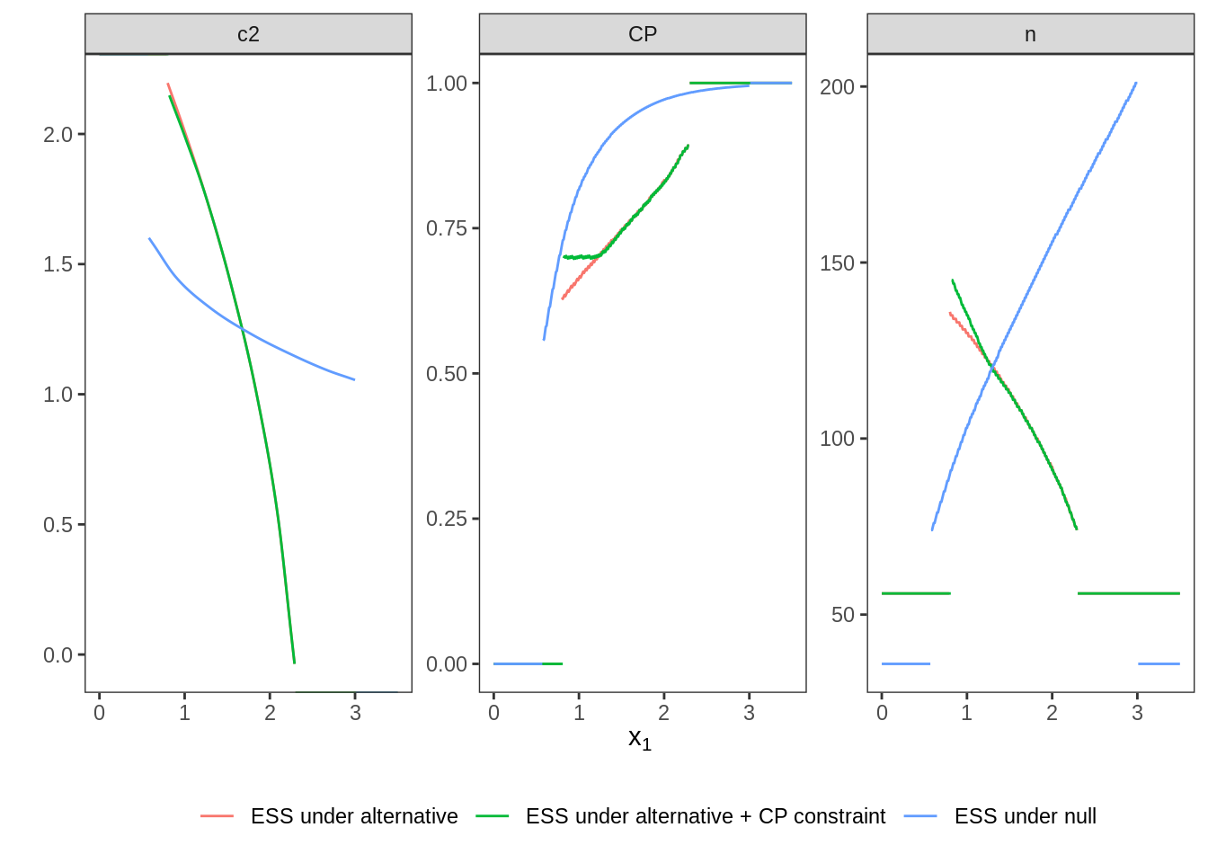
2.5 Plot Two-Stage Designs

The following figure shows the three optimal two-stage designs side by side. The effect of the conditional power constraint (CP not below 0.7) is clearly visible and the very different characteristics between optimizing under the null or the alternative are clearly visible.