5 Scenario IV: smaller effect, point prior

5.1 Details

In this scenario, we return to point priors as investigated in Scenario I. The main goal is to validate adoptr’s sensitivity with regard to the assumed effect size and the constraints on power and type one error rate.

Therefore, we still assume a two-armed trial with normally distributed outcomes. The assumed effect size under the alternative is \(\delta = 0.2\) in this setting. Type one error rate is protected at \(2.5\%\) and the power should be at least \(80\%\). We will vary these values in the variants IV.2 and IV.3

# data distribution and hypotheses
datadist   <- Normal(two_armed = TRUE)
H_0        <- PointMassPrior(.0, 1)
prior      <- PointMassPrior(.2, 1)

# constraints
alpha      <- 0.025
min_power  <- 0.8
toer_cnstr <- Power(datadist, H_0)   <= alpha
pow_cnstr  <- Power(datadist, prior) >= min_power

5.2 Variant IV-1: Minimizing Expected Sample Size under Point Prior

5.2.1 Objective

Expected sample size under the alternative point prior \(\delta = 0.2\) is minimized.

ess <- ExpectedSampleSize(datadist, prior)

5.2.2 Constraints

No additional constraints are considered in this variant.

5.2.3 Initial Design

For this example, the optimal one-stage, group-sequential, and generic two-stage designs are computed. The initial design that is used as starting value of optimization is defined as a group-sequential design by the package rpact that fulfills type one error rate and power constraints in the case of group-sequential and two-stage design. The initial one-stage design is chosen heuristically. The order of integration is set to \(5\).

order <- 5L 

tbl_designs <- tibble(
    type    = c("one-stage", "group-sequential", "two-stage"),
    initial = list(
        OneStageDesign(500, 2.0),
        rpact_design(datadist, 0.2, 0.025, 0.8, TRUE, order),
        TwoStageDesign(rpact_design(datadist, 0.2, 0.025, 0.8, TRUE, order))) )

5.2.4 Optimization

tbl_designs <- tbl_designs %>% 
    mutate(
       optimal = purrr::map(initial, ~minimize(
         
          ess,
          subject_to(
              toer_cnstr,
              pow_cnstr
          ),
          
          initial_design = ., 
          opts           = opts)) )

5.2.5 Test Cases

Firstly, it is checked whether the maximum number of iterations was not exceeded in all three cases.

tbl_designs %>% 
  transmute(
      type, 
      iterations = purrr::map_int(tbl_designs$optimal, 
                                  ~.$nloptr_return$iterations) ) %>%
  {print(.); .} %>% 
  {testthat::expect_true(all(.$iterations < opts$maxeval))}

## # A tibble: 3 × 2
##   type             iterations
##   <chr>                 <int>
## 1 one-stage                20
## 2 group-sequential        959
## 3 two-stage              2096

Now, the constraints on type one error rate and power are tested via simulation.

tbl_designs %>% 
  transmute(
      type, 
      toer  = purrr::map(tbl_designs$optimal, 
                         ~sim_pr_reject(.[[1]], .0, datadist)$prob), 
      power = purrr::map(tbl_designs$optimal, 
                         ~sim_pr_reject(.[[1]], .2, datadist)$prob) ) %>% 
  unnest(., cols = c(toer, power)) %>% 
  {print(.); .} %>% {
  testthat::expect_true(all(.$toer  <= alpha * (1 + tol)))
  testthat::expect_true(all(.$power >= min_power * (1 - tol))) }

## # A tibble: 3 × 3
##   type               toer power
##   <chr>             <dbl> <dbl>
## 1 one-stage        0.0251 0.799
## 2 group-sequential 0.0250 0.800
## 3 two-stage        0.0250 0.800

Due to increasing degrees of freedom, the expected sample sizes under the alternative should be ordered as ‘one-stage > group-sequential > two-stage’. They are evaluated by simulation as well as by evaluate().

tbl_designs %>% 
    mutate(
        ess      = map_dbl(optimal,
                           ~evaluate(ess, .$design) ),
        ess_sim  = map_dbl(optimal,
                           ~sim_n(.$design, .2, datadist)$n ) ) %>%
    {print(.); .} %>% {
    # sim/evaluate same under alternative?
    testthat::expect_equal(.$ess, .$ess_sim, 
                           tolerance = tol_n,
                           scale = 1)
    # monotonicity with respect to degrees of freedom
    testthat::expect_true(all(diff(.$ess) < 0)) }

## # A tibble: 3 × 5
##   type             initial    optimal          ess ess_sim
##   <chr>            <list>     <list>         <dbl>   <dbl>
## 1 one-stage        <OnStgDsg> <adptrOpR [3]>  392     392 
## 2 group-sequential <GrpSqntD> <adptrOpR [3]>  324.    323.
## 3 two-stage        <TwStgDsg> <adptrOpR [3]>  320.    319.

Furthermore, the expected sample size under the alternative of the optimal group-sequential design should be lower than for the group-sequential design by rpact that is based on the inverse normal combination test.

tbl_designs %>%
             filter(type == "group-sequential") %>%
             { expect_lte(
                 evaluate(ess, {.[["optimal"]][[1]]$design}),
                 evaluate(ess, {.[["initial"]][[1]]})
             ) }

Finally, the \(n_2\) function of the optimal two-stage design is expected to be monotonously decreasing:

expect_true(
    all(diff(
        # get optimal two-stage design n2 pivots
        tbl_designs %>% filter(type == "two-stage") %>%
           {.[["optimal"]][[1]]$design@n2_pivots} 
        ) < 0) )

5.3 Variant IV-2: Increase Power

5.3.1 Objective

The objective remains expected sample size under the alternative \(\delta = 0.2\).

5.3.2 Constraints

The minimal required power is increased to \(90\%\).

min_power_2 <- 0.9
pow_cnstr_2 <- Power(datadist, prior) >= min_power_2

5.3.3 Initial Design

For both flavours with two stages (group-sequential, generic two-stage) the initial design is created by rpact to fulfill the error rate constraints.

tbl_designs_9 <- tibble(
    type    = c("one-stage", "group-sequential", "two-stage"),
    initial = list(
        OneStageDesign(500, 2.0),
        rpact_design(datadist, 0.2, 0.025, 0.9, TRUE, order),
        TwoStageDesign(rpact_design(datadist, 0.2, 0.025, 0.9, TRUE, order))) )

5.3.4 Optimization

tbl_designs_9 <- tbl_designs_9 %>% 
    mutate(
       optimal = purrr::map(initial, ~minimize(
         
          ess,
          subject_to(
              toer_cnstr,
              pow_cnstr_2
          ),
          
          initial_design = ., 
          opts           = opts)) )

5.3.5 Test Cases

We start checking if the maximum number of iterations was not exceeded in all three cases.

tbl_designs_9 %>% 
  transmute(
      type, 
      iterations = purrr::map_int(tbl_designs_9$optimal, 
                                  ~.$nloptr_return$iterations) ) %>%
  {print(.); .} %>% 
  {testthat::expect_true(all(.$iterations < opts$maxeval))}

## # A tibble: 3 × 2
##   type             iterations
##   <chr>                 <int>
## 1 one-stage                30
## 2 group-sequential       1485
## 3 two-stage              3069

The type one error rate and power constraints are evaluated by simulation.

tbl_designs_9 %>% 
  transmute(
      type, 
      toer  = purrr::map(tbl_designs_9$optimal, 
                         ~sim_pr_reject(.[[1]], .0, datadist)$prob), 
      power = purrr::map(tbl_designs_9$optimal, 
                         ~sim_pr_reject(.[[1]], .2, datadist)$prob) ) %>% 
  unnest(., cols = c(toer, power)) %>% 
  {print(.); .} %>% {
  testthat::expect_true(all(.$toer  <= alpha * (1 + tol)))
  testthat::expect_true(all(.$power >= min_power_2 * (1 - tol))) }

## # A tibble: 3 × 3
##   type               toer power
##   <chr>             <dbl> <dbl>
## 1 one-stage        0.0251 0.900
## 2 group-sequential 0.0249 0.900
## 3 two-stage        0.0250 0.900

Due to increasing degrees of freedom, the expected sample sizes under the alternative should be ordered as ‘one-stage > group-sequential > two-stage’. This is tested by simulation as well as by evaluate().

tbl_designs_9 %>% 
    mutate(
        ess      = map_dbl(optimal,
                           ~evaluate(ess, .$design) ),
        ess_sim  = map_dbl(optimal,
                           ~sim_n(.$design, .2, datadist)$n ) ) %>%
    {print(.); .} %>% {
    # sim/evaluate same under alternative?
    testthat::expect_equal(.$ess, .$ess_sim, 
                           tolerance = tol_n,
                           scale = 1)
    # monotonicity with respect to degrees of freedom
    testthat::expect_true(all(diff(.$ess)     < 0)) 
    testthat::expect_true(all(diff(.$ess_sim) < 0))}

## # A tibble: 3 × 5
##   type             initial    optimal          ess ess_sim
##   <chr>            <list>     <list>         <dbl>   <dbl>
## 1 one-stage        <OnStgDsg> <adptrOpR [3]>  525     525 
## 2 group-sequential <GrpSqntD> <adptrOpR [3]>  405.    405.
## 3 two-stage        <TwStgDsg> <adptrOpR [3]>  397.    397.

Comparing with the inverse-normal based group-sequential design created by rpact, the optimal group-sequential design should show a lower expected sample size under the point alternative.

tbl_designs_9 %>%
             filter(type == "group-sequential") %>%
             { expect_lte(
                 evaluate(ess, {.[["optimal"]][[1]]$design}),
                 evaluate(ess, {.[["initial"]][[1]]})
             ) }

Since a point prior is regarded, the \(n_2\) function of the optimal two-stage design is expected to be monotonously decreasing:

expect_true(
    all(diff(
        # get optimal two-stage design n2 pivots
        tbl_designs_9 %>% filter(type == "two-stage") %>%
           {.[["optimal"]][[1]]$design@n2_pivots} 
        ) < 0) )

5.4 Variant IV-3: Increase Type One Error rate

5.4.1 Objective

As in variants IV.1 and IV-2, expected sample size under the point alternative is minimized.

5.4.2 Constraints

While the power is still lower bounded by \(90\%\) as in variant II, the maximal type one error rate is increased to \(5\%\).

alpha_2      <- .05
toer_cnstr_2 <- Power(datadist, H_0) <= alpha_2

5.4.3 Initial Design

Again, a design computed by means of the package rpact to fulfill the updated error rate constraints is applied as initial design for the optimal group-sequential and generic two-stage designs.

tbl_designs_5 <- tibble(
    type    = c("one-stage", "group-sequential", "two-stage"),
    initial = list(
        OneStageDesign(500, 2.0),
        rpact_design(datadist, 0.2, 0.05, 0.9, TRUE, order),
        TwoStageDesign(rpact_design(datadist, 0.2, 0.05, 0.9, TRUE, order))) )

5.4.4 Optimization

tbl_designs_5 <- tbl_designs_5 %>% 
    mutate(
       optimal = purrr::map(initial, ~minimize(
         
          ess,
          subject_to(
              toer_cnstr_2,
              pow_cnstr_2
          ),
          
          initial_design = ., 
          opts           = opts)) )

5.4.5 Test Cases

The convergence of the optimization algorithm is tested by checking if the maximum number of iterations was not exceeded.

tbl_designs_5 %>% 
  transmute(
      type, 
      iterations = purrr::map_int(tbl_designs_5$optimal, 
                                  ~.$nloptr_return$iterations) ) %>%
  {print(.); .} %>% 
  {testthat::expect_true(all(.$iterations < opts$maxeval))}

## # A tibble: 3 × 2
##   type             iterations
##   <chr>                 <int>
## 1 one-stage                27
## 2 group-sequential       1070
## 3 two-stage              2208

By simulation, the constraints on the error rates (type one error and power) are tested.

tbl_designs_5 %>% 
  transmute(
      type, 
      toer  = purrr::map(tbl_designs_5$optimal, 
                         ~sim_pr_reject(.[[1]], .0, datadist)$prob), 
      power = purrr::map(tbl_designs_5$optimal, 
                         ~sim_pr_reject(.[[1]], .2, datadist)$prob) ) %>% 
  unnest(., cols = c(toer, power)) %>% 
  {print(.); .} %>% {
  testthat::expect_true(all(.$toer  <= alpha_2 * (1 + tol)))
  testthat::expect_true(all(.$power >= min_power_2 * (1 - tol))) }

## # A tibble: 3 × 3
##   type               toer power
##   <chr>             <dbl> <dbl>
## 1 one-stage        0.0502 0.900
## 2 group-sequential 0.0500 0.900
## 3 two-stage        0.0502 0.900

Due to increasing degrees of freedom, the expected sample sizes under the alternative should be ordered as ‘one-stage > group-sequential > two-stage’. They are tested by simulation as well as by calling evaluate().

tbl_designs_5 %>% 
    mutate(
        ess      = map_dbl(optimal,
                           ~evaluate(ess, .$design) ),
        ess_sim  = map_dbl(optimal,
                           ~sim_n(.$design, .2, datadist)$n ) ) %>%
    {print(.); .} %>% {
    # sim/evaluate same under alternative?
    testthat::expect_equal(.$ess, .$ess_sim, 
                           tolerance = tol_n,
                           scale = 1)
    # monotonicity with respect to degrees of freedom
    testthat::expect_true(all(diff(.$ess) < 0)) }

## # A tibble: 3 × 5
##   type             initial    optimal          ess ess_sim
##   <chr>            <list>     <list>         <dbl>   <dbl>
## 1 one-stage        <OnStgDsg> <adptrOpR [3]>  428     428 
## 2 group-sequential <GrpSqntD> <adptrOpR [3]>  325.    325.
## 3 two-stage        <TwStgDsg> <adptrOpR [3]>  319.    319.

The expected sample size under the alternative that was used as objective criterion of the optimal group-sequential design should be lower than for the group-sequential design by rpact that is based on the inverse normal combination test.

tbl_designs_5 %>%
             filter(type == "group-sequential") %>%
             { expect_lte(
                 evaluate(ess, {.[["optimal"]][[1]]$design}),
                 evaluate(ess, {.[["initial"]][[1]]})
             ) }

Also in this variant, the \(n_2\) function of the optimal two-stage design is expected to be monotonously decreasing:

expect_true(
    all(diff(
        # get optimal two-stage design n2 pivots
        tbl_designs_5 %>% filter(type == "two-stage") %>%
           {.[["optimal"]][[1]]$design@n2_pivots} 
        ) < 0) )

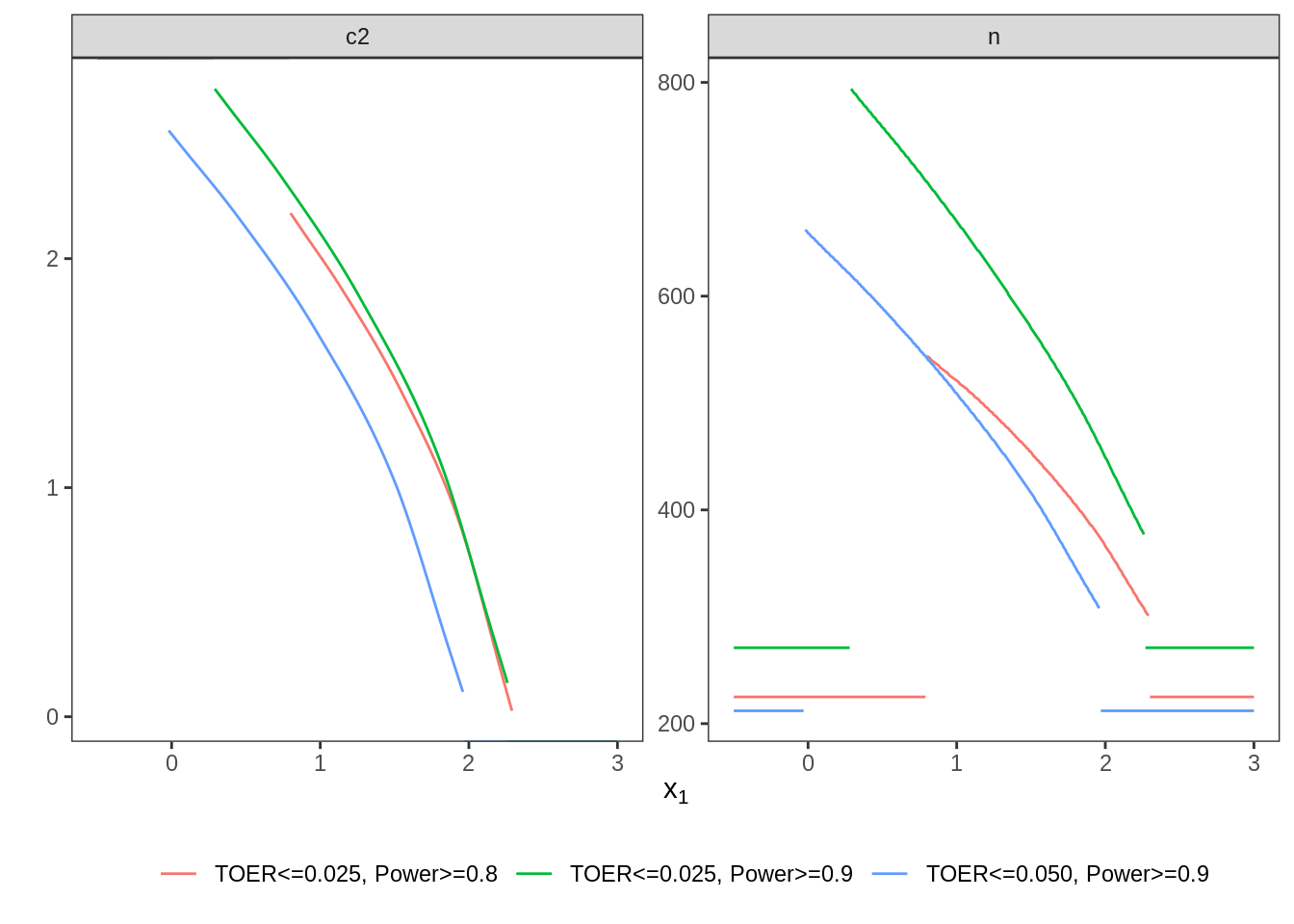
5.5 Plot Two-Stage Designs

The optimal two-stage designs stemming from the three different variants are plotted together.