3 Scenario II: large effect, Gaussian prior

3.1 Details

In this scenario, we revisit the case from Scenario I, but are not assuming a point prior any more. Instead, a Gaussian prior with mean \(\vartheta = 0.4\) and variance \(\tau^2 = 0.2^2\) on the effect size is assumed, i.e.  \(\delta \sim \mathcal{N} (0.4, 0.2^2)\).

In order to fulfill regulatory considerations, the type one error rate is still protected under the point prior \(\delta = 0\) at the level of significance \(\alpha = 0.025\).

The power constraint, however, needs to be modified. It is not senseful to compute the power as rejection probability under the full prior, because effect sizes less than a minimal clinically relevant effect do not show (sufficient) evidence againt the null hypothesis. Therefore, we assume a minimal clinically relevant effect size \(\delta = 0.0\) and condition the prior on values \(\delta > 0\) to compute expected power. In the following, the expected power should be at least \(0.8\).

# data distribution and priors
datadist   <- Normal(two_armed = TRUE)
H_0        <- PointMassPrior(.0, 1)
prior      <- ContinuousPrior(function(delta) dnorm(delta, mean = .4, sd = .2),
                              support = c(-5, 5),
                              tighten_support = TRUE)

# define constraints on type one error rate and expected power
alpha      <- 0.025
min_epower <- 0.8
toer_cnstr <- Power(datadist, H_0) <= alpha
epow_cnstr <- Power(datadist, condition(prior, c(0.0, prior@support[2]))) >= min_epower

3.2 Variant II-1: Minimizing Expected Sample Size under Point Prior

3.2.1 Objective

Expected sample size under the full prior is minimized, i.e., \(\boldsymbol{E}\big[n(\mathcal{D})\big]\).

ess <- ExpectedSampleSize(datadist, prior)

3.2.2 Constraints

No additional constraints are considered in this variant.

3.2.3 Initial Design

For this example, the optimal one-stage, group-sequential, and generic two-stage designs are computed. While the initial design for the one-stage case is determined heuristically, both the group sequential and the generic two-stage designs are optimized starting from the a group-sequential design that is computed by the rpact package to fulfill the type one error rate constraint and that fulfills the power constraint at an effect size of \(\delta = 0.3\).

order <- 5L
# data frame of initial designs 
tbl_designs <- tibble(
    type    = c("one-stage", "group-sequential", "two-stage"),
    initial = list(
        OneStageDesign(250, 2.0),
        rpact_design(datadist, 0.3, 0.025, 0.8, TRUE, order),
        TwoStageDesign(rpact_design(datadist, 0.3, 0.025, 0.8, TRUE, order))) )

The order of integration is set to 5.

3.2.4 Optimization

For all these three initial designs, the resulting optimal designs are computed.

tbl_designs <- tbl_designs %>% 
    mutate(
       optimal = purrr::map(initial, ~minimize(
         
          ess,
          subject_to(
              toer_cnstr,
              epow_cnstr
          ),
          
          initial_design = ., 
          opts           = opts)) )

3.2.5 Test Cases

Firstly, it is checked that the maximum number of iterations was not reached in all these cases.

tbl_designs %>% 
  transmute(
      type, 
      iterations = purrr::map_int(tbl_designs$optimal, 
                                  ~.$nloptr_return$iterations) ) %>%
  {print(.); .} %>% 
  {testthat::expect_true(all(.$iterations < opts$maxeval))}

## # A tibble: 3 × 2
##   type             iterations
##   <chr>                 <int>
## 1 one-stage                26
## 2 group-sequential        720
## 3 two-stage              1965

Since type one error rate is defined under the point effect size \(\delta=0\), the type one error rate constraint can be tested for all three optimal designs.

tbl_designs %>% 
  transmute(
      type, 
      toer = purrr::map(tbl_designs$optimal, 
                        ~sim_pr_reject(.[[1]], .0, datadist)$prob) ) %>% 
  unnest(., cols = c(toer)) %>% 
  {print(.); .} %>% {
  testthat::expect_true(all(.$toer <= alpha * (1 + tol))) }

## # A tibble: 3 × 2
##   type               toer
##   <chr>             <dbl>
## 1 one-stage        0.0251
## 2 group-sequential 0.0250
## 3 two-stage        0.0249

Since the optimal two-stage design is more flexible than the optimal group-sequential design (constant \(n_2\) function) and this is more flexible than the optimal one-stage design (no second stage), the expected sample sizes under the prior should be ordered in the opposite way. Additionally, expected sample sizes under the null hypothesis are computed both via evaluate() and simulation-based.

essh0 <- ExpectedSampleSize(datadist, H_0)

tbl_designs %>% 
    mutate(
        ess       = map_dbl(optimal,
                            ~evaluate(ess, .$design) ),
        essh0     = map_dbl(optimal,
                            ~evaluate(essh0, .$design) ),
        essh0_sim = map_dbl(optimal,
                            ~sim_n(.$design, .0, datadist)$n ) ) %>% 
    {print(.); .} %>% {
    # sim/evaluate same under null?
    testthat::expect_equal(.$essh0, .$essh0_sim, 
                           tolerance = tol_n,
                           scale = 1)
    # monotonicity with respect to degrees of freedom
    testthat::expect_true(all(diff(.$ess) < 0)) }

## # A tibble: 3 × 6
##   type             initial    optimal          ess essh0 essh0_sim
##   <chr>            <list>     <list>         <dbl> <dbl>     <dbl>
## 1 one-stage        <OnStgDsg> <adptrOpR [3]>  165   165       165 
## 2 group-sequential <GrpSqntD> <adptrOpR [3]>  117.  115.      115.
## 3 two-stage        <TwStgDsg> <adptrOpR [3]>  115.  119.      119.

3.3 Variant II-2: Minimizing Expected Sample Size under Null Hypothesis

3.3.1 Objective

Expected sample size conditioned on negative effect sizes is minimized, i.e.,

ess_0 <- ExpectedSampleSize(datadist, condition(prior, c(bounds(prior)[1], 0)))

3.3.2 Constraints

No additional constraints besides type one error rate and expected power are considered in this variant.

3.3.3 Initial Design

As in Variant I.2 another initial design is more appropriate for optimization under the null hypothesis. In this situation, one may expect a different (increasing) sample size function, and thus also a different shape of the \(c_2\) function. Therefore, the rpact initial design is a suboptimal starting point. Instead, we start with a constant \(c_2\) function by heuristically setting it to \(2\) on the continuation area. Since optimization under the null hypothesis favours extremely conservative boundaries for early efficacy stopping we impose as quite liberal upper bound of \(3\) for early efficacy stopping.

init_design_h0 <- tbl_designs %>% 
    filter(type == "two-stage") %>% 
    pull(initial) %>% 
    .[[1]]
init_design_h0@c2_pivots <- rep(2, order)

ub_design <- TwoStageDesign(
    3 * init_design_h0@n1,
    2,
    3,
    rep(600, order),
    rep(3.0, order)
)

3.3.4 Optimization

opt_neg <- minimize(
  
        ess_0,
        
        subject_to(
          
            toer_cnstr,
            epow_cnstr
        ),
        
        initial_design = init_design_h0,
        upper_boundary_design = ub_design,
        opts = opts
)

3.3.5 Test Cases

First of all, check if the optimization algorithm converged. To avoid improper solutions, it is first verified that the maximum number of iterations was not exceeded in any of the three cases.

testthat::expect_true(opt_neg$nloptr_return$iterations < opts$maxeval)
print(opt_neg$nloptr_return$iterations)

## [1] 7197

Again, the type one error rate under the point null hypothesis \(\delta = 0\) can be tested by simulation.

tbl_toer <- tibble(
  toer     = evaluate(Power(datadist, H_0), opt_neg$design),
  toer_sim = sim_pr_reject(opt_neg$design, .0, datadist)$prob
)

print(tbl_toer)

## # A tibble: 1 × 2
##     toer toer_sim
##    <dbl>    <dbl>
## 1 0.0249   0.0250

testthat::expect_true(tbl_toer$toer <= alpha * (1 + tol))
testthat::expect_true(tbl_toer$toer_sim <= alpha * (1 + tol))

Furthermore, the expected sample size under the prior conditioned on negative effect sizes (\(\delta \leq 0\)) should be lower for the optimal design derived in this variant than for the optimal design from Variant II.1 where expected sample size under the full prior was minimized.

testthat::expect_lte(
    evaluate(ess_0, opt_neg$design),
    evaluate(
        ess_0, 
        tbl_designs %>% 
            filter(type == "two-stage") %>% 
            pull(optimal) %>% 
            .[[1]] %>% 
            .$design )
)

3.4 Variant II-3: Conditional Power Constraint

3.4.1 Objective

As in Variant II-1, expected sample size under the full prior is minimized.

3.4.2 Constraints

In addition to the constraints on type one error rate and expected power, a constraint on conditional power to be larger than \(0.7\) is included.

cp       <- ConditionalPower(datadist, condition(prior, c(0, prior@support[2])))
cp_cnstr <- cp >= 0.7

3.4.3 Initial Design

The previous initial design can still be applied.

3.4.4 Optimization

opt_cp <- minimize(
        ess,
        subject_to(
            toer_cnstr,
            epow_cnstr,
            cp_cnstr
        ),
        initial_design = tbl_designs$initial[[3]],
        opts = opts
)

3.4.5 Test Cases

We start checking whether the maximum number of iterations was not reached.

print(opt_cp$nloptr_return$iterations)

## [1] 2012

testthat::expect_true(opt_cp$nloptr_return$iterations < opts$maxeval)

The type one error rate is tested via simulation and compared to the value obtained by evaluate().

tbl_toer <- tibble(
  toer     = evaluate(Power(datadist, H_0), opt_cp$design),
  toer_sim = sim_pr_reject(opt_cp$design, .0, datadist)$prob
)

print(tbl_toer)

## # A tibble: 1 × 2
##     toer toer_sim
##    <dbl>    <dbl>
## 1 0.0250   0.0250

testthat::expect_true(tbl_toer$toer <= alpha * (1 + tol))
testthat::expect_true(tbl_toer$toer_sim <= alpha * (1 + tol))

The conditional power is evaluated via numerical integration on several points inside the continuation region and it is tested whether the constraint is fulfilled on all these points.

tibble(
    x1 = seq(opt_cp$design@c1f, opt_cp$design@c1e, length.out = 25),
    cp = map_dbl(x1, ~evaluate(cp, opt_cp$design, .)) ) %>% 
  {print(.); .} %>% {
      testthat::expect_true(all(.$cp >= 0.7 * (1 - tol))) }

## # A tibble: 25 × 2
##       x1    cp
##    <dbl> <dbl>
##  1 0.675 0.698
##  2 0.747 0.700
##  3 0.819 0.700
##  4 0.891 0.699
##  5 0.963 0.698
##  6 1.03  0.698
##  7 1.11  0.701
##  8 1.18  0.705
##  9 1.25  0.709
## 10 1.32  0.715
## # … with 15 more rows

Due to the additional constraint in comparison to Variant II.1, Variant II.3 should show a larger expected sample size under the prior than Variant II.1

testthat::expect_gte(
    evaluate(ess, opt_cp$design),
    evaluate(
        ess, 
        tbl_designs %>% 
            filter(type == "two-stage") %>% 
            pull(optimal) %>% 
            .[[1]] %>% 
            .$design )
)

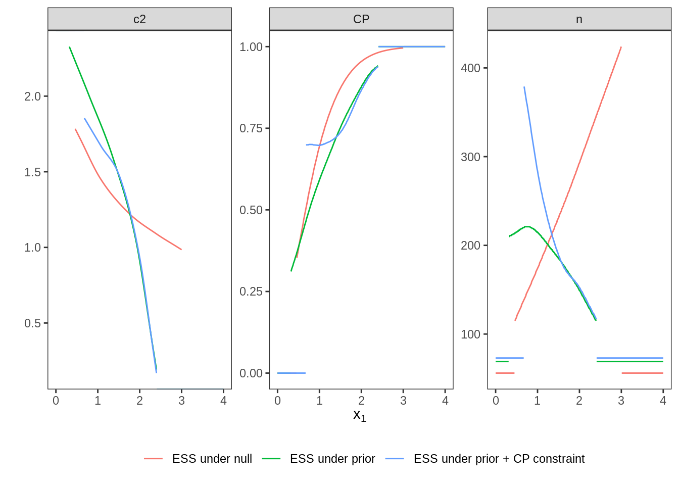
3.5 Plot Two-Stage Designs

The optimal two-stage designs stemming from the different variants are plotted together.