4 Scenario III: large effect, uniform prior

4.1 Details

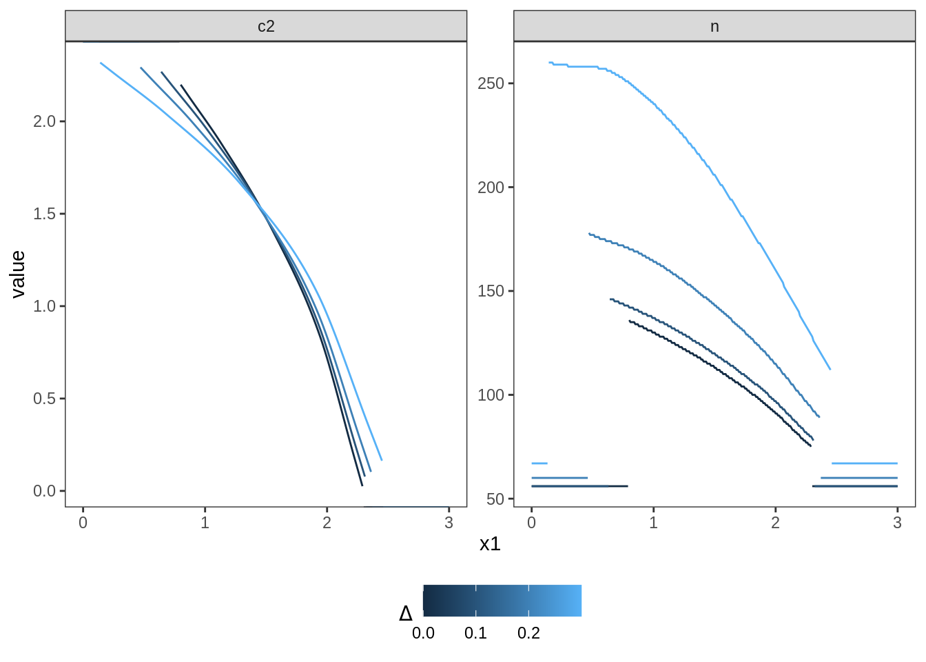
This scenario covers a similar setting as Scenario I. The purpose is to asses whether placing uniform priors with decreasing width of support centered at \(\delta=0.4\) leads to a sequence of optimal designs which converges towards the solution in variant I-1.

The trial is still considered to be two-armed with normally distribtuted outcomes and the type one error rate under the null hypothesis \(\mathcal{H}_0:\delta \leq 0\) is to be protected at \(\alpha = 0.025\).

datadist   <- Normal(two_armed = TRUE)
H_0        <- PointMassPrior(.0, 1)
alpha      <- 0.025
toer_cnstr <- Power(datadist, H_0) <= alpha

In this scenario we consider a sequence of uniform distributions \(\delta\sim\operatorname{Unif}(0.4 - \Delta_i, 0.4 + \Delta_i)\) around \(0.4\) with \(\Delta_i=(3 - i)/10\) for \(i=0\ldots 3\). I.e., for \(\Delta_3=0\) reduces to PointMassPrior on \(\delta=0.4\).

prior <- function(delta) {
    if (delta == 0)
        return(PointMassPrior(.4, 1.0))
    a <- .4 - delta; b <- .4 + delta
    ContinuousPrior(function(x) dunif(x, a, b), support = c(a, b))
}

Across all variants in this scenario, the expected power under the respective prior conditioned on \(\delta > 0\) must be at least \(0.8\). I.e., throughout this scenario, we always use the following constraint on expected power.

ep_cnstr <- function(delta) {
    prior     <- prior(delta)
    cnd_prior <- condition(prior, c(0, bounds(prior)[2]))
    return( Power(datadist, cnd_prior) >= 0.8 )
}

4.2 Variant III.1: Convergence under prior concentration

The goal of this variant is to make sure that the optimal solution converges as the prior is more and more concentrated at a point mass.

4.2.1 Objective

Expected sample size under the respective prior is minimized, i.e., \(\boldsymbol{E}\big[n(\mathcal{D})\big]\).

objective <- function(delta) {
    ExpectedSampleSize(datadist, prior(delta))
}

4.2.2 Constraints

The constraints have already been described under details.

4.2.3 Optimization problem

The optimization problem depending on \(\Delta_i\) is defined below. The default optimization parameters, 5 pivot points, and a fixed initial design are used. The initial design is chosen such that the error constraints are fulfilled. Early stopping for futility is applied if the effect shows in the opponent direction to the alternative, i.e. \(c_1^f=0\). \(c_2\) is chosen close to and \(c_1^e\) a little larger than the \(1-\alpha\)-quantile of the standard normal distribution. The sample sizes are selected to fulfill the error constraints.

init <- TwoStageDesign(
    n1    = 150,
    c1f   = 0,
    c1e   = 2.3,
    n2    = 125.0,
    c2    = 2.0,
    order = 5
)

optimal_design <- function(delta) {
    minimize(
        objective(delta),
        subject_to(
            toer_cnstr,
            ep_cnstr(delta)
        ),
        initial_design = init
    )
}

# compute the sequence of optimal designs
deltas  <- 3:0/10
results <- lapply(deltas, optimal_design)

4.2.4 Test cases

Check that iteration limit was not exceeded in any case.

iters <- sapply(results, function(x) x$nloptr_return$iterations)
print(iters)

## [1] 2368 1891 2685 2789

testthat::expect_true(all(iters <= opts$maxeval))

Check type one error rate control by simulation and by calling evaluate().

df_toer <- tibble(
  delta    = deltas,
  toer     = sapply(results, function(x) evaluate(Power(datadist, H_0), x$design)),
  toer_sim = sapply(results, function(x) sim_pr_reject(x$design, .0, datadist)$prob)
)

testthat::expect_true(all(df_toer$toer     <= alpha * (1 + tol)))
testthat::expect_true(all(df_toer$toer_sim <= alpha * (1 + tol)))

print(df_toer)

## # A tibble: 4 × 3
##   delta   toer toer_sim
##   <dbl>  <dbl>    <dbl>
## 1   0.3 0.0250   0.0250
## 2   0.2 0.0250   0.0250
## 3   0.1 0.0250   0.0250
## 4   0   0.0250   0.0250

Check that expected sample size decreases with decreasing prior variance.

testthat::expect_gte(
  evaluate(objective(deltas[1]), results[[1]]$design),
  evaluate(objective(deltas[2]), results[[2]]$design)
)

testthat::expect_gte(
  evaluate(objective(deltas[2]), results[[2]]$design),
  evaluate(objective(deltas[3]), results[[3]]$design)
)

testthat::expect_gte(
  evaluate(objective(deltas[3]), results[[3]]$design),
  evaluate(objective(deltas[4]), results[[4]]$design)
)

4.2.5 Plot designs

Finally, we plot the designs and assess for convergence.