The adoptr Package: Adaptive Optimal Designs for Clinical Trials in R

Kevin Kunzmann

Cambridge University
kevin.kunzmann@mrc-bsu.cam.ac.uk

Maximilian Pilz

University of Heidelberg
pilz@imbi.uni-heidelberg.de

Carolin Herrmann

Charité Berlin and Berlin Insitute of Health
carolin.herrmann@charite.de

Geraldine Rauch

Charité Berlin and Berlin Insitute of Health
geraldine.rauch@charite.de

Meinhard Kieser

University of Heidelberg
meinhard.kieser@imbi.uni-heidelberg.de

2023-04-17

Abstract

Even though adaptive two-stage designs with unblinded interim analyses are becoming increasingly popular in clinical trial designs, there is a lack of statistical software to make their application more straightforward. The package adoptr fills this gap for the common case of two-stage one- or two-arm trials with (approximately) normally distributed outcomes. In contrast to previous approaches, adoptr optimizes the entire design upfront which allows maximal efficiency. To facilitate experimentation with different objective functions, adoptr supports a flexible way of specifying both (composite) objective scores and (conditional) constraints by the user. Special emphasis was put on providing measures to aid practitioners with the validation process of the package.

This manuscript was accepted for publication in the Journal of Statistical Software.

Background

Confirmatory clinical trials are conducted in a strictly regulated environment. A key quality criterion put forward by the relevant agencies (US Food and Drug Administration and others (2019), Committee for Medicinal Products for Human Use and others (2007)) for a study that is supposed to provide evidence for the regulatory acceptance of a new drug or treatment is strict type one error rate control. This requirement was often seen as conflicting with the perceived need to make trials more flexible by, e.g., early stopping for futility, group-sequential enrollment, or even adaptive sample size recalculation. An excellent historical review of the development of the field of adaptive clinical trial designs and the struggles along the way is given in Bauer et al. (2015).

In this manuscript, the focus lies exclusively on adaptive two-stage designs with one unblinded interim analysis. Both early stopping for futility and efficacy are allowed and the final sample size as well as the critical value to reject the null hypothesis is chosen in a data-driven way. There is a plethora of methods for modifying the design of an ongoing trial based on interim results without compromising type one error rate control (Bauer et al. 2015) but the criteria for deciding which adaptation should be performed during an interim analysis and when to perform the interim analysis are still widely based on heuristics. Bauer et al. mention this issue of guiding adaptive decisions at interim in a principled (i.e., ‘optimal’) way by stating that ‘[t]he question might arise if potential decisions made at interim stages might not be better placed to the upfront planning stage.’ Following Mehta and Pocock (2011), Jennison and Turnbull (2015) developed a principle approach to optimal interim sample size modifications, i.e., to conduct the interim decision (conditional on interim results) such that it optimizes an unconditional performance score. Their approach, however, was still restricted unnecessarily. Recently, Pilz et al. (2019) extended the work to a fully general variational problem where the optimization problem for any given performance score (optionally under further constraints) is solved over both the sample size adaptation function and the critical value function and the time point of the interim decision simultaneously. This approach is an application of ideas which have been put forward in single-arm trials with binary endpoint for several years (Englert and Kieser (2013), Kunzmann and Kieser (2016), Kunzmann and Kieser (2020)) to a setting with continuous test statistics. Clearly, by relaxing the problem to continuous sample sizes and test statistics, the theory becomes much more tractable, and important connections between conditional and unconditional optimality can be discussed much easier (Pilz et al. 2019).

A key insight from this recent development is the fact that the true challenge in designing an adaptive trial is less the technical methodology for controlling the type one error rate but rather the choice of the optimality criterion. This issue is much less pressing in single-stage designs since most sensible criteria will be equivalent to minimizing the overall sample size. Thus, in this case, a ‘design’ is often completely specified by given power and type one error rate constraints. For the more complex adaptive designs, however, there are much more sensible criteria (minimize maximal sample size, expected sample size, expected costs, etc.) and the balance between conditional and unconditional properties must be explicitly specified (cf. Section 6). This added complexity might be seen as daunting by practitioners, but it is also a chance for tailoring adaptive designs more specifically to a particular situation. The R-package (R Core Team 2019) adoptr aims at providing a simple yet customizable interface to specifying a broad class of objective functions and constraints for single- or two-arm, one- or two-stage designs with approximately normally distributed endpoints. The goal of adoptr is to enable relatively easy experimentation with different notions of optimality to shift the focus from how to optimize to what to optimize.

In the following, we first give a definition of the problem setting addressed in adoptr and the technicalities of translating the underlying variational problem to a simple multivariate optimization problem before motivating the need for an R-package. We then present the core functionality of adoptr before addressing the issue of facilitating validation of open-source software in a regulated environment and discussing potential future work on adoptr.

Setting

We consider the problem of a two-stage, two-arm design to establish superiority of treatment over placebo with respect to the mean difference. Assume that to that end data \(Y_j^{g, i}\) is observed for the \(j\)-th individual of the trial in stage \(i\in\{1,2\}\) under treatment (\(g=T\)) or placebo (\(g=C\)). Let \(n_i\) be the per-group sample size in stage \(i\) and consider the stage-wise test statistics \[ X_i := \frac{\sum_{j=1}^{n_i}Y_j^{T,i} - \sum_{j=1}^{n_i}Y_j^{C,i}}{\sigma\,\sqrt{2\,n_i}} \] for \(i=1,2\). Under the assumption that the \(Y_j^{g, i}\stackrel{iid}{\sim} F_g\) with \(\boldsymbol{E}[F_T] - \boldsymbol{E}[F_C] = \theta\) and common variance \(\sigma^2\), by the central limit theorem, the asymptotic distribution of \(X_1\) is \(\mathcal{N}(\sqrt{n_1/2}\, \theta, 1)\). Formally, the null hypothesis for the superiority test is thus \(\mathcal{H}_0:\theta\leq 0\). Based on the interim outcome \(X_1\), a decision can be made whether to either stop the trial early for futility if \(X_1<c_1^f\), to stop the trial early for efficacy (early rejection of the null hypothesis) if \(X_1>c_1^e\), or to enter stage two if \(X_1\in[c_1^f, c_1^e]\). Conditional on proceeding to a second stage, it holds that \(X_2\,|\,X_1\in[c_1^f, c_1^e]\sim\mathcal{N}(\sqrt{n_2/2}\, \theta, 1)\). In the second stage, the null hypothesis is rejected if and only if \(X_2 > c_2(X_1)\) for a stage-two critical value \(c_2:x_1\mapsto c_2(x_1)\). To test \(\mathcal{H}_0\) at a significance level of \(\alpha\), the stage-one critical values \(c_1^f\) and \(c_1^e\) as well as \(c_2(\cdot)\) must be chosen in a way that protects the overall maximal type one error rate \(\alpha\). Note that it is convenient to define \(c_2(x_1) = \infty\) if \(x_1<c_1^f\) and \(c_2(x_1) = -\infty\) if \(x_1>c_1^e\) since the power curve of the design is then given by \(\theta\mapsto\boldsymbol{Pr}_\theta\big[X_2>c_2(X_1)\big]\). This results in a classical group-sequential design and several methods were proposed in the literature for choosing the early-stopping boundaries \(c_1^f\) and \(c_1^e\) (O’Brien and Fleming (1979), Pocock (1977)) and for defining the stage-two rejection boundary function \(c_2(\cdot)\) (Bauer and Köhne (1994), Hedges and Olkin (1985)). Often, the inverse-normal combination test (Lehmacher and Wassmer 1999) is applied and \(c_2(\cdot)\) is defined as a linear function of the stage-one test-statistic \[ c_2(x_1) = \frac{c - w_1 x_1}{w_2}‚ \] for a critical value \(c\) and predefined weights \(w_1\) and \(w_2\). Most commonly, the stage-wise test statistics are weighted in terms of their respective sample sizes, i.e., \(w_1 = \sqrt{n_1 / (n_1+n_2)}\) and \(w_2 = \sqrt{n_2 / (n_1+n_2)}\). This choice of the weights is optimal in the sense that it minimizes the variance of the final test statistic if the assumed sample sizes are indeed realized (Zaykin 2011). Note, however, that such prespecified weights become inefficient if the sample size deviates strongly from the anticipated value (cf. Wassmer and Brannath (2016), chapter 6.2.5). A natural extension of this group-sequential framework is to allow the second stage sample size to also depend on the observed interim outcome, i.e., to consider a function \(n_2:x_1\mapsto n_2(x_1)\) instead of a fixed value \(n_2\). Such ‘adaptive’ two-stage designs are thus completely characterized by a five-tuple \(\mathcal{D}:=\big(n_1, c_1^f, c_1^e, n_2(\cdot), c_2(\cdot)\big)\).

While the required sample size and the critical value for a single-stage design are uniquely defined by given type one error rate and power constraints, it is much less clear how the design parameters of a two-stage design should be selected. This is especially true since both \(n_2\) and \(c_2\) are functions and thus the parameter space is in fact infinite-dimensional. In order to compare different choices of the design parameters, appropriate scoring criteria are essential. A widely applied criterion is the expected sample size under the alternative hypothesis (see, e.g., Jennison and Turnbull (2015)). However, there is a variety of further scoring criteria that could be incorporated or even combined in order to rate a two-stage design. For instance, conditional power is defined as the probability to reject the null hypothesis under the alternative given the interim result \(X_1=x_1\): \[ \operatorname{CP}_\theta(x_1) := \boldsymbol{Pr}_\theta \big[X_2 > c_2(X_1) \, \big| \, X_1=x_1\big]. \] Hence, conditional power is a conditional score given as the power conditioned on the first-stage outcome \(X_1=x_1\). Vice versa, power can be seen as an unconditional score that is obtained by integrating conditional power over all possible stage-one outcomes, i.e., \[ \operatorname{Power_\theta} = \boldsymbol{E}_\theta\big[\operatorname{CP}(X_1)\big]. \] Intuitively, it makes sense to require a minimal conditional power upon continuation to the second stage since one might otherwise continue a trial with little prospect of still rejecting the null hypothesis. We demonstrate the consequences of this heuristic in Section 6.4. Once the scoring criterion is selected, the design parameters may be chosen in order to optimize this objective. The first ones to address this problem were Jennison and Turnbull (2015) who minimized the expected sample size \[ \text{ESS}_{\theta}(\mathcal{D}) := \boldsymbol{E}_{\theta} \big[n(X_1) \big] := \boldsymbol{E}_{\theta} \big[n_1 + n_2(X_1) \big] \] of a two-stage design for given \(n_1,c_1^f, c_1^e\) with respect to \(n_2(\cdot)\) for given power and type one error rate constraints. The function \(c_2(\cdot)\), however, was not optimized. Instead, Jennison and Turnbull (2015) used a combination test approach to derive \(c_2\) given \(n_2(\cdot)\) and \(n_1\) (cf. Equation @ref(eq:inverse-normal)). In Pilz et al. (2019), the authors demonstrated that this restriction is not necessary and that the variational problem of deriving both functions \(n_2(\cdot)\) and \(c_2(\cdot)\) given \(n_1,c_1^f, c_1^e\) to minimize expected sample size can be solved by analyzing the corresponding Euler-Lagrange equation. Nesting this step in a standard optimization over the stage-one parameters allows identifying an optimal set of all design parameters without imposing parametric assumptions on \(c_2(\cdot)\). As a result, a fully optimal design \(\mathcal{D}^*:=\big(n_1^*, c_1^{f,*}, c_1^{e, *}, n_2^*(\cdot), c_2^*(\cdot)\big)\) for the following general optimization problem was derived \[\begin{align} & \text{minimize} && \operatorname{ESS}_{\theta_1}(\mathcal{D}) &&&& \\ & \text{subject to:} && \boldsymbol{Pr}_{\theta_0}\big[X_2>c_2(X_1)\big] &&\leq \alpha, &&&& \\ &&& \boldsymbol{Pr}_{\theta_1}\big[X_2>c_2(X_1)\big] &&\geq 1-\beta &&&& \end{align}\] where \(\theta_0=0\).

Direct variational perspective

In adoptr, a simpler solution strategy than solving the Euler-Lagrange equation locally is applied to the same problem class. We propose to embed the entire problem in a finite-dimensional parameter space and solve the corresponding problem over both stage-one and stage-two design parameters simultaneously using standard numerical libraries. I.e., we adopt a direct approach to solving the variational problem. This is done by defining a discrete set of pivot points \(\widetilde{x}_1^{(i)}\in(c_1^f, c_1^e), i=1,\ldots,k\), and interpolating \(c_2\) and \(n_2\) between these pivots. We use cubic Hermite splines (Fritsch and Carlson 1980) which are sufficiently flexible, even for a moderate number of pivots, to approximate any realistic stage-two sample size and critical value functions. Since the optimal functions are generally very smooth (Pilz et al. 2019) they are well suited to spline interpolation. Within the adoptr validation report (cf. Section 7) we investigate empirically the shape of the approximated functions and that increasing the number of pivots above a value of 5 to 7 does not improve the optimization results. The latter implies that a relatively small number of pivot points appears to be sufficient to obtain valid spline approximations of the optimal functions. Note that the pivots are only needed in the continuation region since both functions are (piecewise) constant within the early stopping regions. In adoptr, the pivots are defined as nodes of a Gaussian quadrature rule of degree \(k\). This choice allows fast and precise numerical integration of any conditional score over the continuation region, e.g., \[\begin{align} \text{ESS}_{\theta}(\mathcal{D}) = \int n(x_1) f_{\theta} (x_1) \operatorname{d} x_1 \approx n_1 + \sum_{i=1}^{k} \omega_i\, n_2\big(\widetilde{x}_1^{(i)}\big) f_{\theta} \big(\widetilde{x}_1^{(i)}\big), \end{align}\] where \(f_\theta\) is the probability density function of \(X_1\,|\,\theta\) and \(\omega_i\) are the corresponding weights of the integration rule. The weights only depend on \(k\) and the nodes just need to be scaled to the integration interval. Consequentially, this objective function is smooth in the optimization parameters and the resulting optimization problem is of dimension \(2k+3\), where the tuning parameters are \(\big(n_1, c_1^f, c_1^e, n_2\big(\widetilde{x}_1^{(1)}\big), \dots, n_2\big(\widetilde{x}_1^{(k)}\big), c_2\big(\widetilde{x}_1^{(1)}\big), \dots, c_2\big(\widetilde{x}_1^{(k)}\big)\big)\). Standard numerical solvers may then be employed to minimize it. Since adoptr enables generic objectives (cf. Section 6.3), it uses the gradient-free optimizer COBYLA (Powell 1994) internally via the R-package nloptr (Johnson (2018), Ypma, Borchers, and Eddelbuettel (2018)).

Most commonly used unconditional performance scores \(S(\mathcal{D})\) can be seen as expected values over conditional scores \(S(\mathcal{D}|X_1)\) by \(S(\mathcal{D}) = \boldsymbol{E}\big[S(\mathcal{D}|X_1)\big]\) in a similar way as power and expected sample size. Any such ‘integral score’ can be computed quickly and reliably in adoptr via the choice of pivots outlined above. The correctness of numerically integrated scores is checked in the adoptr validation report by comparing the numerical integrals to simulated results.

Note that we tacitly relaxed all sample sizes to be real numbers in the above argument while they are in fact restricted to positive integers. Integer-valued \(n_1\) and \(n_2\) would, however, lead to an NP-hard mixed-integer problem. In our experiments, we found that merely rounding both \(n_1\) and \(n_2\) after the optimization works fine. The extensive validation suite (cf. Section 7) evaluates by numerical integration and simulation whether the included constraints are fulfilled for optimal designs with rounded sample sizes. Up to now, neither the constraints were violated nor an efficiency loss with respect to the underlying objective function was observed. In theory, one could re-adjust the decision boundaries for these rounded sample sizes, but we failed to see any practical benefit from this, even for small trials where the rounding error is largest (data not shown).

The need for an R package

Bauer et al. (2015) state that adequate statistical software for adaptive designs ‘is increasingly needed to evaluate the adaptations and to find reasonable strategies’.

Commercial software such as JMP (SAS Institute Inc., n.d.a) or Minitab (Minitab, Inc. 2020) allow planning and analyzing a wide range of experimental setups. Amongst others, they provide tools for randomization, stratification, block-building, or D-optimal designs. These general purpose statistical software packages do not, however, allow planning of more specialized multi-stage designs encountered in clinical trials. For group-sequential designs, some planning capabilities are available in the SAS procedure seqdesign (SAS Institute Inc., n.d.b), PASS (NCSS 2019), or ADDPLAN (ICON plc 2020). East (Cytel 2020) also supports design, simulation and analysis of experiments with interim analyses. The East ADAPT and the East SURVADAPT modules support sample size recalculation. Furthermore, there are various open-source R-packages for the analysis of multi-stage designs. The package adaptTest (Vandemeulebroecke 2009) implements combination tests for adaptive two-stage designs. AGSDest (Hack, Brannath, and Brueckner 2019) allows estimation and computation of confidence intervals in adaptive group-sequential designs. More detailed overviews on software for adaptive clinical trial designs can be found in Bauer et al. (2015), chapter 6, or in Tymofyeyev (2014). The choice of software for optimally designing two- or multi-stage designs, however, is much more limited. Current R-packages concerned with optimal clinical trial designs are OptGS (Wason and Burkardt (2015), Wason (2015)) and rpact (Wassmer and Pahlke 2019). These are, however, exclusively focused on group-sequential designs and lack the ability to specify custom objective functions and constraints.

The lack of flexibility in formulating the objective function and constraints might lead to off-the-shelf solutions not entirely reflecting the needs of a particular trial consequentially resulting in inefficient designs. The R-package adoptr aims at providing a simple and interactive yet flexible interface for addressing a range of optimization problems encountered with two-stage one- or two-arm clinical trials. In particular, adoptr allows to model a priori uncertainty over \(\theta\) via prior distributions and thus supports optimization under uncertainty (cf. Section 6.2). adoptr also supports the combination of conditional (on \(X_1\)) and unconditional scores and constraints to address concerns such as type-one-error-rate control (unconditional score) and, e.g., a minimal conditional power (conditional score) simultaneously (cf. Section 6.3). To facilitate the adoption of these advanced trial designs in the clinical trials community, adoptr also features an extensive test and validation suite (cf. Section 7).

In the following, we outline the key design principles for adoptr.

1. Interactivity: A major advantage of the R-programming language is its powerful metaprogramming capabilities and flexible class system. With a combination of non-standard evaluation and S4 classes, we hope to achieve a structured and modular way of expressing optimization problems in clinical trials that integrates nicely with an interactive workflow. We feel that a step-wise problem formulation via the creation of modular intermediate objects, which can be explored and modified separately, encourages exploration of different options.
2. Reliability: A crux in open-source software development for clinical trials is achieving demonstrable validation. Potential users need to be convinced of the software quality and need to be able to comply with their respective validation requirements which often require the ability to produce a validation report. This burden typically results in innovative software not being used at all - simply because the validation effort cannot be stemmed. We address this issue with an extensive unit test suite and a companion validation report (cf. Section 7).
3. Extensibility: We do not want to impose a particular choice of scores or constraints or promote a particular notion of optimality for clinical trial designs. In cases where the composition of existing scores is not sufficient, the object-oriented approach of adoptr facilitates the definition of custom scores and constraints that seamlessly integrate with the remainder of the package.

Adoptr’s structure

The package adoptr is based on R’s S4 class system. This allows to use multiple dispatch on the classes of multiple arguments to a method. In this section, the central components of adoptr are described briefly. Figure @ref(fig:class-diagram) gives a structural overview of the main classes in adoptr.

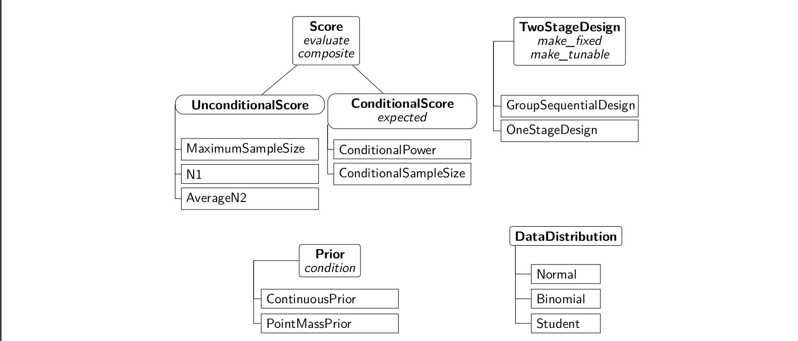
Overview of the most important classes and methods (in italic) in the R-package adoptr. A subclassing relationship is indicated by a connecting line to the corresponding super class above it. The most important methods for each class are listed under the respective class name in italic font.

To compute optimal designs, an object of class UnconditionalScore must be defined as objective criterion. adoptr distinguishes between ConditionalScores and UnconditionalScores (cf. Section 2). All Scores can be evaluated using the method evaluate. For unconditional scores, this method only requires a Score object and a TwoStageDesign object, for conditional scores (like conditional power), it also requires the interim outcome \(x_1\). Note that any ConditionalScore \(S(\mathcal{D}|X_1=x_1)\) can be converted to an UnconditionalScore \(S(\mathcal{D}) = \boldsymbol{E}\big[S(\mathcal{D}|X_1)\big]\) using the method expected. The two most widely used conditional scores are pre-implemented as ConditionalPower and ConditionalSampleSize. Their unconditional counterparts are Power and ExpectedSampleSize. Further predefined unconditional scores are MaximumSampleSize, evaluating the maximum sample size, N1, measuring the first-stage sample size, and AverageN2, evaluating the average of the stage-two sample size (improper prior). These scores may be used for regularization if variable stage-two sample sizes or a high stage-one sample size are to be penalized. Users are free to define their own Scores (cf. the vignette ‘Defining New Scores’ (Kunzmann and Pilz 2020)). Moreover, different Scores can be composed to a single one by the function composite (cf. Section 6.3). Both conditional and unconditional scores can also be used to define constraints - the most common case being constraints for power and maximal type one error rate. The function minimize takes an unconditional score as objective and a set of constraints and optimizes the design parameters.

In adoptr, different kinds of designs are implemented. The most frequently applied case is a TwoStageDesign, i.e., a design with one interim analysis and a sample size function that varies with the interim test statistic. Another option is the subclass GroupSequentialDesign which restricts the sample size function on the continuation region to a single number, i.e., \({n_2(x_1) = n_2\ \forall x_1\in[\,c_1^f, c_1^e\,]}\). Additionally, adoptr supports the computation of optimal OneStageDesigns, i.e., designs without an interim analysis. Technically, one-stage designs are implemented as subclasses of TwoStageDesign since they can be viewed as the limiting case for \(n_2\equiv0\) and \(c_1^f=c_1^e\). Hence, all methods that are implemented for TwoStageDesigns also work for GroupSequentialDesigns and OneStageDesigns. Users can chose to keep some elements of a design fixed during optimization using the methods make_fixed (cf. Section 6.5).

The joint data distribution in adoptr consists of two elements. The distribution of the test statistic is specified by an object of class DataDistribution. Currently, the three options Normal, Binomial, and Student are implemented. The logical variable two_armed allows the differentiation between one- and two-armed trials. Furthermore, adoptr supports prior distributions on the effect size. These can be PointMassPriors (cf. Section 6.1) as well as ContinuousPriors (cf. Section 6.2).

In the following section, more hands on examples demonstrate the capabilities of adoptr and its syntax.

Examples

Standard case

Consider the case of a randomized controlled clinical trial where efficacy is to be demonstrated in terms of superiority of the treatment over placebo with respect to the population mean difference \(\theta\) of an outcome. Let the null hypothesis be \(\mathcal{H}_0:\theta\leq 0\). Assume that the maximal type one error rate is to be controlled at a one-sided level \(\alpha=2.5\%\) and a minimal power of \(90\%\) at a point alternative of \(\theta_1=0.3\) is deemed necessary. For simplicity’s sake, we assume \(\sigma^2=1\) without loss of generality. The required sample size for a one-stage design with analysis by the one-sided two-sample \(t\)-test would then be roughly 235 per group.

Using adoptr, the two-stage design minimizing the expected sample size under the alternative hypothesis can be derived for the very same situation. First, the data distribution is specified to be normal. The two_armed parameter allows to switch between single-armed and two-armed trials.

R> datadist <- Normal(two_armed = TRUE)

In this example, we use simple point priors for both the null and alternative hypotheses. The hypotheses and the corresponding scores (power values) can be specified as:

R> null        <- PointMassPrior(theta = .0, mass = 1.0)
R> alternative <- PointMassPrior(theta = .3, mass = 1.0)
R> power       <- Power(dist = datadist, prior = alternative)
R> toer        <- Power(dist = datadist, prior = null)
R> mss         <- MaximumSampleSize()

A Power score requires the data distribution and the prior to be specified. For this example, we choose PointMassPriors with the entire probability mass of \(1\) on a single point, the null hypothesis \(\theta = 0\) to compute the type one error rate, and the alternative hypothesis \(\theta = 0.3\) to compute the power. The objective function is the expected sample size under the alternative.

R> ess <- ExpectedSampleSize(dist = datadist, prior = alternative)

Since adoptr internally relies on the COBYLA implementation of nloptr, an initial design is required. A heuristic initial choice is provided by the function get_initial_design. It is based on a fixed design that fulfills constraints on type one error rate and power. The type of the design (two-stage, group-sequential, or one-stage) and the data distribution have to be defined. For the Gaussian quadrature used during optimization, one also has to specify the order of the integration rule, i.e., the number of pivot points between early stopping for futility and early stopping for efficacy. In practice, order 7 turned out to be sufficiently flexible to obtain valid results (data not shown).

R> initial_design <- get_initial_design(theta = 0.3, alpha = 0.025,
+                                       beta = 0.1, type = "two-stage",
+                                       dist = datadist, order = 7)

It is easy to check that the initial design does not fulfill any of the constraints (minimal power of 90% and maximal type one error rate of 2.5%) with equality by evaluating the respective scores:

R> evaluate(toer, initial_design)

## [1] 0.0246875

R> evaluate(power, initial_design)

## [1] 0.8130973

Alternatively, one might also evaluate a constraint object directly via

R> evaluate(toer  <= .025, initial_design)

## [1] -0.0003125

R> evaluate(power >= .9, initial_design)

## [1] 0.08690272

All constraint objects are normalized to the form \(h(\mathcal{D}) \leq 0\) (unconditional) or \(h(\mathcal{D}, x_1) \leq 0\) (conditional on \(X_1=x_1\)). Calling evaluate on a constraint object then simply returns the left-hand side of the inequality. The actual optimization is started by invoking minimize

R> opt1 <- minimize(ess, subject_to(power >= 0.9, toer  <= 0.025),
+                   initial_design)

The modular structure of the problem specification is intended to facilitate the inspection or modification of individual components. The call to minimize() is designed to be as close as possible to the mathematical formulation of the optimization problem and returns both the optimized design (opt1$design) as well as the full nloptr return value with details on the optimization procedure (opt1$nloptr_return).

A summary method for objects of the class TwoStageDesign is available to quickly evaluate a set of ConditionalScores such as conditional power as well as UnconditionalScores such as power and expected sample size.

R> cp <- ConditionalPower(dist = datadist, prior = alternative)
R> summary(opt1$design, "Power" = power, "ESS" = ess, "CP" = cp)

## TwoStageDesign: n1 = 120 
## 
          futility |                  continue                 | efficacy
## 
      x1:     0.28 |  0.33  0.54  0.87  1.27  1.68  2.01  2.22 |  2.27
## 
  c2(x1):     +Inf | +2.70 +2.53 +2.23 +1.82 +1.31 +0.74 +0.19 |  -Inf
## 
  n2(x1):        0 |   229   214   188   154   116    79    51 |     0
## 
  CP(x1):     0.00 |  0.69  0.72  0.75  0.79  0.83  0.87  0.91 |  1.00
## 
   Power:      0.899
## 
     ESS:    176.126
## 

adoptr also implements a default plot method for the overall sample size and the stage-two critical value as functions of the first-stage test statistic \(x_1\). The plot method also accepts additional ConditionalScores such as conditional power. Calling the plot method produces several plots with the interim test statistic \(x_1\) on the \(x\)-axis and the respective function on the \(y\)-axis.

R> plot(opt1$design, `Conditional power` = cp)

Optimal sample size, critical value, and conditional power plotted against the interim test statistic (built-in plot method).

Note the slightly bent shape of the \(c_2(\cdot)\) function (cf. Figure @ref(fig:standard-case), second plot). For two-stage designs based on the inverse-normal combination function, \(c_2(\cdot)\) would be linear by definition (cf. Equation @ref(eq:inverse-normal)). Since the optimal shape of \(c_2(\cdot)\) is not linear (but almost), inverse-normal combination methods are slightly less efficient (cf. Pilz et al. (2019) for a more detailed discussion of this issue).

Optimization under uncertainty

adoptr is not limited to point priors but also supports arbitrary continuous prior distributions. Consider the same situation as before but now assume that the prior over the effect size is given by a much more realistic truncated normal distribution with mean \(0.3\) and standard deviation \(0.1\), i.e., \(\theta\sim\mathcal{N}_{[-1, 1]}(0.3, 0.1^2)\). The order of integration is set to 25 to obtain precise results.

R> prior <- ContinuousPrior(
+    pdf     = function(theta) dnorm(theta, mean = .3, sd = .1),
+    support = c(-1, 1),
+    order   = 25)

The objective function is the expected sample size under the prior

R> ess <- ExpectedSampleSize(dist = datadist, prior = prior)

and we replace power with expected power \[ \boldsymbol{E} \Big[ \boldsymbol{Pr}_\theta\big[X_2>c_2(X_1)\big] \, \Big| \, \theta \geq 0.1 \Big] \] which is the expected power given a relevant effect (here we define the minimal relevant effect as \(0.1\)). This score can be defined in adoptr by first conditioning the prior.

R> epower <- Power(dist = datadist, prior = condition(prior, c(.1, 1)))

The optimal design under the point prior only achieves an expected power of

R> evaluate(epower, opt1$design)

## [1] 0.8143914

The optimal design under the truncated normal prior fulfilling the expected power constraint is then given by

R> opt2 <- minimize(ess, subject_to(epower >= 0.9, toer <= 0.025),
+                   initial_design,
+                   opts = list(algorithm = "NLOPT_LN_COBYLA",
+                               xtol_rel = 1e-5, maxeval = 20000))

Note that the increased complexity of the problem requires a larger maximal number of iterations for the underlying optimization procedure. adoptr exposes the nloptr options via the argument opts. In cases where the maximal number of iterations is exhausted, a warning is thrown.

The expected sample size under the prior of the obtained optimal design equals 236.2. This shows that an increased uncertainty on \(\theta\) requires larger sample sizes to fulfill the expected power constraint since the expected sample size under the continuous prior considered in this section of the optimal design derived under a point alternative (see Section 6.1) is only 176.4.

Utility maximization and composite scores

adoptr also supports composite scores. This can be used to derive utility maximizing designs by defining an objective function combining both expected power and expected sample size instead of imposing a hard constraint on expected power. For example, in the above situation one could be interested in a utility-maximizing design. Here, we consider the utility function \[ u(\mathcal{D}) := 200000\, \boldsymbol{E} \Big[ \boldsymbol{Pr}_\theta\big[X_2>c_2(X_1)\big] \, \Big| \, \theta \geq 0.1 \Big] - \boldsymbol{E}\Big[n(X_1)^2\Big], \] thus allowing a direct trade-off between power and sample size. Here, the expected sample size is chosen because the practitioner might prefer flatter sample size curves. This can be achieved with expected squared sample size by penalizing large sample sizes stronger than low sample sizes. Furthermore, there is no longer a strict expected power constraint but the expected power becomes part of the utility function which allows a direct trade-off between the two quantities. This can be interpreted as a pricing mechanism (cf. Kunzmann and Kieser (2020)): Every additional percent point of expected power has a (positive) value of \(\$ 2'000\) while an increase of \(\boldsymbol{E}\big[n(X_1)^2\big]\) by \(1\) incurs costs of \(\$ 1\). The goal is then to compute the design which is maximizing the overall utility defined by the utility function \(u(\mathcal{D})\) (or equivalently minimize costs).

A composite score can be defined via any valid numerical R expression of score objects. We start by defining a score for the expected quadratic sample size

R> `n(X_1)`      <- ConditionalSampleSize()
R> `E[n(X_1)^2]` <- expected(composite({`n(X_1)`^2}),
+                            data_distribution = datadist,
+                            prior = prior)

before minimizing the corresponding negative utility without a hard expected power constraint.

R> opt3 <- minimize(composite({`E[n(X_1)^2]` - 200000*epower}),
+                   subject_to(toer <= 0.025), initial_design)

The expected power of the design is

R> evaluate(epower, opt3$design)

## [1] 0.796554

The three optimal designs which have been computed so far are depicted in a joint plot (cf. Figure @ref(fig:comparison)). The design using the continuous prior requires higher sample sizes due to the higher uncertainty about \(\theta\). The utility maximization approach results in similar shapes of \(n(\cdot)\) and \(c_2(\cdot)\) as the constraint optimization. However, the sample sizes are lower due to the design’s lower power which is only possible by allowing a trade-off between expected power and expected sample size. In particular, the maximal sample size of the utility-based design equals 256 and is distinctly smaller than in the case of a hard power constraint under a point prior (maximal sample size: 352) or a continuous prior (maximal sample size: 527).

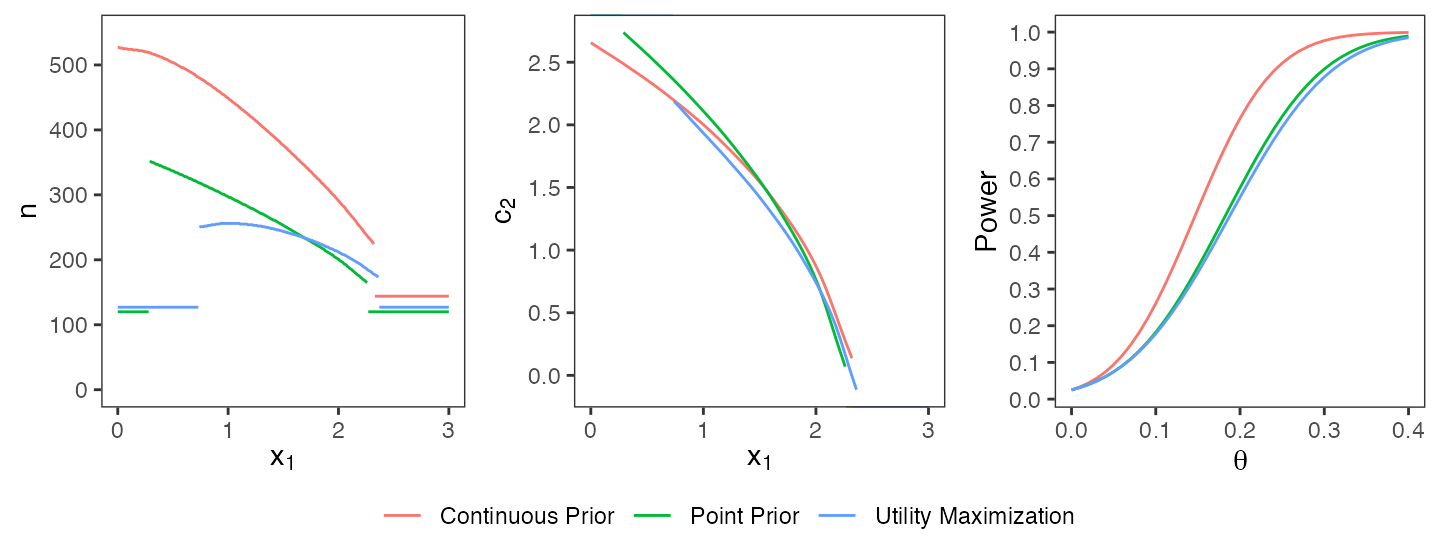
Comparison of optimal designs under a point prior, a continuous prior, and a utility maximization approach.

Conditional power constraint

adoptr also allows the incorporation of hard constraints on conditional scores such as conditional power. Conditional power constraints are intuitively sensible to make sure that a trial which continues to the second stage maintains a high chance of rejecting the null hypothesis at the end. For this example, we return to the case of a point prior on the effect size.

R> prior <- PointMassPrior(theta = .3, mass = 1.0)
R> ess   <- ExpectedSampleSize(dist = datadist, prior = prior)
R> cp    <- ConditionalPower(dist = datadist, prior = prior)
R> power <- expected(cp, data_distribution = datadist, prior = prior)

Here, power is derived as expected score of the corresponding conditional power. A conditional power constraint is added in exactly the same way as unconditional constraints.

R> opt4 <- minimize(ess, subject_to(toer <= 0.025, power >= 0.9, cp >= 0.8),
+                   initial_design)

Comparing the optimal design that has been computed here with the same constraints but without a conditional power constraint (cf. beginning of this chapter), the optimal design with the additional constraint requires larger sample sizes in regions where the conditional power would usually be below the given threshold (cf. Figure @ref(fig:cp-constraint), first and third plot). Overall, the additional constraint reduces the feasible solution space and consequently increases the expected sample size (176.6 with conditional power constraint vs. 176.1 without). This example demonstrates, that any additional binding conditional constraints do come at costs for global optimality. Whether or not the loss in unconditional performance is outweighed by more appealing conditional properties must be decided on a case by case basis.

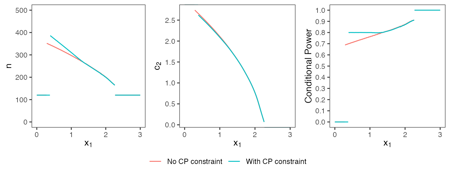
Optimal designs with and without conditional power constraint.

Keeping design parameters fixed

In clinical practice, non-statistical considerations may impose direct constraints on design parameters. For instance, a sponsor might be subject to logistical constraints that render it necessary to design a trial with a specific stage one sample size. Returning to the standard case discussed in Section 6.1, assume that a stage-one per-group sample size of exactly 80 individuals per group is required (\(n_1 = 80\)) instead of the optimal value of \(n_1^* = 120\). Furthermore, assume that the sponsor wants to stop early for futility if and only if there is a negative effect size at the interim analysis, i.e., \(c_1^f = 0\). adoptr supports such considerations by allowing to fix specific values of a design:

R> initial_design@n1  <- 80
R> initial_design@c1f <- 0
R> initial_design     <- make_fixed(initial_design, n1, c1f)

Any ‘fixed’ parameter will be kept constant during optimization. Note that it is also possible to ‘un-fix’ parameters again using the make_tunable function.

R> opt5 <- minimize(ess, subject_to(toer <= 0.025, power >= 0.9),
+                   initial_design)

Figure @ref(fig:tunable) visually compares the original design with the new, more restricted design. The designs are qualitatively similar, but fixing \(n_1\) and \(c_1^f\) does come at the price of slightly increased expected sample size (187.7 compared to 176.1 in the less restricted case).

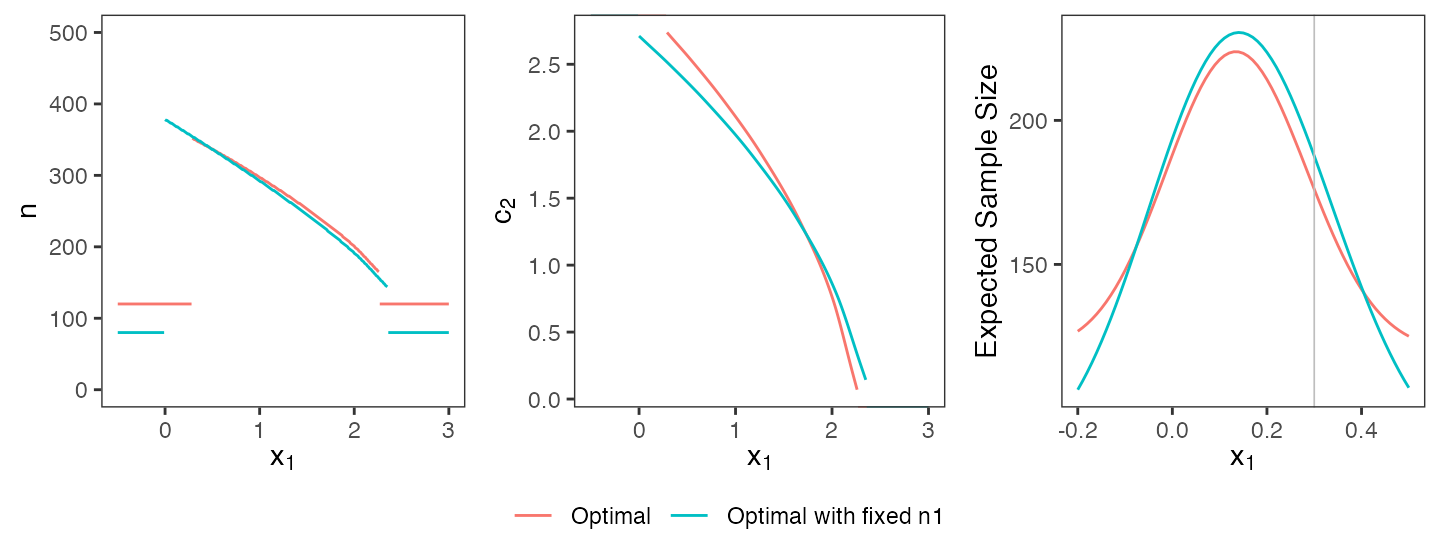
Comparison of fully optimal design and optimal design with fixed first-stage sample size.

Validation concept

The conduct and analysis of clinical trials is a highly regulated process. An essential requirement being put forward in Title 21 CRF (code of federal regulations) Part 11 is the need to validate any software used to work with or produce records (US Food and Drug Administration and others 2003). The exact scope of regulations such as CRF 11 is sometimes difficult to assess, and it is not always clear which regulations apply to R packages used in a production environment (The R Foundation for Statistical Computing 2013). Irrespective of the applicability of the CRF 11 to adoptr, the design of a clinical trial is undoubtedly crucial and package authors should provide extensive evidence of the correctness of the package functionality. Additionally, this evidence should be easily accessible and human-readable. The latter requirement is a consequence of the fact that, again following CRF 11 and the remarks in The R Foundation for Statistical Computing (2013), a ‘validated R-package’ does not exist since the validation process must always be implemented by the responsible user.

To facilitate the process of validation as much as possible, adoptr implements the following measures:

1. Open-source development: The entire development of adoptr is organized around a public GitHub.com repository (https://github.com/kkmann/adoptr). Anybody can freely download the source code, browse the development history, raise issues, or contribute to the code base by opening pull requests.
2. CRAN releases: Regular CRAN (CRAN 2020) releases of updated versions maximize visibility and add an additional layer of testing and quality control. New features can be implemented and tested in the (public) development version on GitHub before pushing new releases to CRAN.
3. Unit testing: adoptr implements an extensive test suite using the package testthat (Wickham, R Studio, and R Core Team (2018), Wickham (2011)) which allows spotting new errors early during development and localizing them quickly. Together with continuous integration (cf. below), this helps to improve quality and speeds up the development process.
4. Continuous Integration / Continuous Deployment: adoptr makes extensive use of the continuous integration and deployment services GitHub Actions (GitHub.com 2021). Each new commit on the public GitHub.com repository is immediately run through the automated testing pipeline. Merges to the master branch are only possible after tests were passed successfully and a contributor reviewed and approved the changes (‘branch protection system’). Continuous deployment allows automatically updating code-coverage statistics (cf. below) and up-to-date online documentation (cf. below).
5. Coverage analyses: To document the extent to which the test suite covers the package code, adoptr relies on the codecov (Codecov LLC 2020) online service in conjunction with the covr package (Hester 2019). It provides statistics on the proportion of lines visited at least once during testing (currently 100%) and enables easy online publication of the results.
6. Online documentation: Beyond the standard documentation generated using roxygen2 (Hadley Wickham et al. 2019), we also make use of the pkgdown (H. Wickham and Hesselberth 2019) package and the free GitHub pages service to publish a static html version of the documentation online at https://kkmann.github.io/adoptr/. This includes both the function reference and the vignettes in a consistent and easily accessible format. The online documentation experience is further improved by the integration of a full-text docsearch engine (https://www.algolia.com/ref/docsearch).
7. Extended validation report: There are limits to what can be done in the standard unit testing framework within a package itself (cf. https://cran.r-project.org/web/packages/policies.html). Long-running test suites also hinder active development with a strict continuous integration and continuous deployment (CI/CD) workflow since changes to the master branch require passing the automated tests. We, therefore, decided to restrict the internal unit tests to a bare minimum with a clear focus on coverage and technical integrity of the package. To demonstrate correctness of our results over a larger set of examples and in comparison with existing packages such as rpact, we implemented an external ‘validation report’ (sources: https://github.com/kkmann/adoptr-validation-report, current report: https://kkmann.github.io/adoptr-validation-report/) using the bookdown (Xie (2019), Xie (2016)) package. The report itself again uses CI/CD and daily rebuilds to automatically deploy the report corresponding to the most current CRAN-hosted version of the package. Within the report, we still use testthat to conduct formal tests. In case any of these tests fails, the build of the report will fail, the maintainers will get notified, and the status indicator in the repository changes.

Validating the software employed may well be as much work as developing it in the first place. The opaque requirements and the lack of adequate tools to automate validation tasks are a major hurdle for academic developers to address validation issues. The additional work, however, is worth it since it not only improves quality but also facilitates collaboration and makes it easier to promote packages for real-world use.

Future work

The main motivation of implementing adoptr in R is the fact that this is by far the most common programming language used by the target audience. Note, however, that using R for generic nonlinear constraint optimization problems leads to a performance bottleneck since there is currently no stable and efficient way of obtaining gradient information for generic, user-defined functions. Since one of the design principles of adoptr is extensibility, the ability to support custom objective functions is central. In R, this implies that one has to resort to either a finite differences approximation of first- and second-order derivatives or to a completely gradient-free optimizer such as COBYLA. In our experiments, we found that COBYLA was far more stable than a finite-differences augmented Lagrangian method (data not shown). Still, for some problems, convergence using COBYLA is rather slow. An interesting alternative to R and nloptr would therefore be Julia (Bezanson et al. 2017) and the JuMP framework for numerical programming (Lubin and Dunning 2015). This framework allows interfacing generic nonlinear solvers via a common interface and, leveraging Julia’s excellent automatic-differentiation capabilities, is able to provide fast and precise (second-order) gradient information for user-defined objective functions.

Acknowledgments

The first two authors contributed equally to this manuscript.

This work was partly supported by the Deutsche Forschungsgemeinschaft under Grant number KI 708/4-1.

References

Bauer, P., F. Bretz, V. Dragalin, F. König, and G. Wassmer. 2015. “Twenty-Five Years of Confirmatory Adaptive Designs: Opportunities and Pitfalls.” Statistics in Medicine 35 (3): 325–47. https://doi.org/10.1002/sim.6472.

Bauer, P., and K. Köhne. 1994. “Evaluation of Experiments with Adaptive Interim Analyses.” Biometrics 50 (4): 1029–41.

Bezanson, J., A. Edelman, S. Karpinski, and V. Shah. 2017. “Julia: A Fresh Approach to Numerical Computing.” SIAM Review 59 (1): 65–98. https://doi.org/10.1137/141000671.

Codecov LLC. 2020. Codecov. https://about.codecov.io/.

Committee for Medicinal Products for Human Use and others. 2007. “Reflection Paper on Methodological Issues in Confirmatory Clinical Trials Planned with an Adaptive Design.” London: EMEA. https://www.ema.europa.eu/en/methodological-issues-confirmatory-clinical-trials-planned-adaptive-design.

CRAN. 2020. Comprehensive R Archive Network. https://cran.r-project.org/.

Cytel. 2020. East 6. https://www.cytel.com/software/east/.

Englert, S., and M. Kieser. 2013. “Optimal Adaptive Two-Stage Designs for Phase Ii Cancer Clinical Trials.” Biometrical Journal 55: 955–68. https://doi.org/10.1002/bimj.201200220.

Fritsch, F. N., and R. E. Carlson. 1980. “Monotone Piecewise Cubic Interpolation.” SIAM Journal on Numerical Analysis 17 (2): 238–46. https://doi.org/10.1137/0717021.

GitHub.com. 2021. GitHub Actions. https://docs.github.com/en/actions/.

Hack, N., W. Brannath, and M. Brueckner. 2019. AGSDest: Estimation in Adaptive Group Sequential Trials. https://CRAN.R-project.org/package=AGSDest.

Hedges, L., and I. Olkin. 1985. Statistical Methods in Meta-Analysis. Academic Press.

Hester, Jim. 2019. Covr: Test Coverage for Packages. https://CRAN.R-project.org/package=covr.

ICON plc. 2020. ADDPLAN. https://www.iconplc.com/innovation/addplan/.

Jennison, C., and B. W. Turnbull. 2015. “Adaptive Sample Size Modification in Clinical Trials: Start Small Then Ask for More?” Statistics in Medicine 34 (29): 3793–3810. https://doi.org/10.1002/sim.6575.

Johnson, S. G. 2018. The Nlopt Nonlinear-Optimization Package. https://nlopt.readthedocs.io/en/latest/.

Kunzmann, K., and M. Kieser. 2016. “Optimal Adaptive Two-Stage Designs for Single-Arm Trial with Binary Endpoint.” arXiv, 1605.00249.

———. 2020. “Optimal Adaptive Single-Arm Phase Ii Trials Under Quantified Uncertainty.” Journal of Biopharmaceutical Statistics 30 (1): 89–103. https://doi.org/10.1080/10543406.2019.1609016.

Kunzmann, K., and M. Pilz. 2020. Defining New Scores. https://rdrr.io/cran/adoptr/f/vignettes/defining-new-scores.Rmd.

Lehmacher, W., and G. Wassmer. 1999. “Adaptive Sample Size Calculations in Group Sequential Trials.” Biometrics 55 (4): 1286–90. https://doi.org/10.1111/j.0006-341X.1999.01286.x.

Lubin, M., and I. Dunning. 2015. “Computing in Operations Research Using Julia.” INFORMS Journal on Computing 27 (2): 238–48. https://doi.org/10.1287/ijoc.2014.0623.

Mehta, C. R., and S. J. Pocock. 2011. “Adaptive Increase in Sample Size When Interim Results Are Promising: A Practical Guide with Examples.” Statistics in Medicine 30 (28): 3267–84. https://doi.org/10.1002/sim.4102.

Minitab, Inc. 2020. Minitab 19 Statistical Software . https://www.minitab.com.

NCSS. 2019. PASS Sample Size 2019 . https://www.ncss.com/software/pass/.

O’Brien, P. C., and T. R. Fleming. 1979. “A Multiple Testing Procedure for Clinical Trials.” Biometrics 35 (3): 549–56.

Pilz, M., K. Kunzmann, C. Herrmann, G. Rauch, and M. Kieser. 2019. “A Variational Approach to Optimal Two-Stage Designs.” Statistics in Medicine 38 (21): 4159–71. https://doi.org/10.1002/sim.8291.

Pocock, S. J. 1977. “Group Sequential Methods in the Design and Analysis of Clinical Trials.” Biometrika 64 (2): 191–99. https://doi.org/10.1093/biomet/64.2.191.

Powell, M. J. D. 1994. “A Direct Search Optimization Method That Models the Objective and Constraint Functions by Linear Interpolation.” In Advances in Optimization and Numerical Analysis, 51–67. Dordrecht: Springer-Verlag Netherlands. https://doi.org/10.1007/978-94-015-8330-5_4.

R Core Team. 2019. R: A Language and Environment for Statistical Computing. Vienna, Austria: The R Foundation for Statistical Computing. https://www.R-project.org/.

SAS Institute Inc., NC, Cary. n.d.a. JMP Clinical .

———. n.d.b. SAS.

The R Foundation for Statistical Computing. 2013. “R: Regulatory Compliance and Validation Issues - a Guidance Document for the Use of R in Regulated Clinical Trial Environments.” https://www.r-project.org/doc/R-FDA.pdf.

Tymofyeyev, Y. 2014. “A Review of Available Software and Capabilities for Adaptive Designs.” In Practical Considerations for Adaptive Trial Design and Implementation, 139–55. Springer-Verlag New York. https://doi.org/10.1007/978-1-4939-1100-4_8.

US Food and Drug Administration and others. 2003. “Guidance for Industry Part 11, Electronic Records; Electronic Signatures — Scope and Application.” US Food Drug Admin, Rockville. https://www.fda.gov/media/75414/download.

US Food and Drug Administration, and others. 2019. Adaptive Designs for Clinical Trials of Drugs and Biologics - Guidance for Industry. https://www.fda.gov/media/78495/download.

Vandemeulebroecke, M. 2009. AdaptTest: Adaptive Two-Stage Tests. https://CRAN.R-project.org/package=adaptTest.

Wason, J. M. S. 2015. “OptGS: An R Package for Finding Near-Optimal Group-Sequential Designs.” Journal of Statistical Software 66 (2): 1–13. https://doi.org/10.18637/jss.v066.i02.

Wason, J. M. S., and J. Burkardt. 2015. OptGS: Near-Optimal and Balanced Group-Sequential Designs for Clinical Trials with Continuous Outcomes. https://CRAN.R-project.org/package=OptGS.

Wassmer, G., and W. Brannath. 2016. Group Sequential and Confirmatory Adaptive Designs in Clinical Trials. Springer Series in Pharmaceutical Statistics -. Springer International Publishing. https://doi.org/10.1007/978-3-319-32562-0.

Wassmer, G., and F. Pahlke. 2019. Rpact: Confirmatory Adaptive Clinical Trial Design and Analysis. https://CRAN.R-project.org/package=rpact.

Wickham, H. 2011. “Testthat: Get Started with Testing.” The R Journal 3: 5–10. https://doi.org/10.32614/RJ-2011-002.

Wickham, Hadley, Peter Danenberg, Gábor Csárdi, and Manuel Eugster. 2019. Roxygen2: In-Line Documentation for R. https://CRAN.R-project.org/package=roxygen2.

Wickham, H., and J. Hesselberth. 2019. Pkgdown: Make Static Html Documentation for a Package. https://CRAN.R-project.org/package=pkgdown.

Wickham, H., R Studio, and R Core Team. 2018. Testthat: Unit Testing for R. https://CRAN.R-project.org/package=testthat.

Xie, Y. 2016. Bookdown: Authoring Books and Technical Documents with R Markdown. Boca Raton, Florida: Chapman; Hall/CRC. https://doi.org/10.1201/9781315204963.

———. 2019. Bookdown: Authoring Books and Technical Documents with R Markdown. https://github.com/rstudio/bookdown.

Ypma, J., H. W. Borchers, and D. Eddelbuettel. 2018. Nloptr: R Interface to Nlopt. https://CRAN.R-project.org/package=nloptr.

Zaykin, D. V. 2011. “Optimally Weighted Z-Test Is a Powerful Method for Combining Probabilities in Meta-Analysis.” Journal of Evolutionary Biology 24 (8): 1836–41. https://doi.org/10.1111/j.1420-9101.2011.02297.x.